Note
Click here to download the full example code
Repeated measures ANOVA on source data with spatio-temporal clustering
This example illustrates how to make use of the clustering functions for arbitrary, self-defined contrasts beyond standard t-tests. In this case we will tests if the differences in evoked responses between stimulation modality (visual VS auditory) depend on the stimulus location (left vs right) for a group of subjects (simulated here using one subject’s data). For this purpose we will compute an interaction effect using a repeated measures ANOVA. The multiple comparisons problem is addressed with a cluster-level permutation test across space and time.
# Authors: Alexandre Gramfort <alexandre.gramfort@inria.fr>
#          Eric Larson <larson.eric.d@gmail.com>
#          Denis Engemannn <denis.engemann@gmail.com>
#
# License: BSD (3-clause)

import os.path as op
import numpy as np
from numpy.random import randn
import matplotlib.pyplot as plt

import mne
from mne.stats import (spatio_temporal_cluster_test, f_threshold_mway_rm,
                       f_mway_rm, summarize_clusters_stc)

from mne.minimum_norm import apply_inverse, read_inverse_operator
from mne.datasets import sample

print(__doc__)
Set parameters
data_path = sample.data_path()
raw_fname = data_path + '/MEG/sample/sample_audvis_filt-0-40_raw.fif'
event_fname = data_path + '/MEG/sample/sample_audvis_filt-0-40_raw-eve.fif'
subjects_dir = data_path + '/subjects'
src_fname = subjects_dir + '/fsaverage/bem/fsaverage-ico-5-src.fif'

tmin = -0.2
tmax = 0.3  # Use a lower tmax to reduce multiple comparisons

#   Setup for reading the raw data
raw = mne.io.read_raw_fif(raw_fname)
events = mne.read_events(event_fname)
Out:
Opening raw data file /home/circleci/mne_data/MNE-sample-data/MEG/sample/sample_audvis_filt-0-40_raw.fif...
    Read a total of 4 projection items:
        PCA-v1 (1 x 10²)  idle
        PCA-v2 (1 x 10²)  idle
        PCA-v3 (1 x 10²)  idle
        Average EEG reference (1 x 60)  idle
    Range : 6450 ... 48149 =     42.956 ...   320.665 secs
Ready.
Read epochs for all channels, removing a bad one
raw.info['bads'] += ['MEG 2443']
picks = mne.pick_types(raw.info, meg=True, eog=True, exclude='bads')
# we'll load all four conditions that make up the 'two ways' of our ANOVA

event_id = dict(l_aud=1, r_aud=2, l_vis=3, r_vis=4)
reject = dict(grad=1000e-13, mag=4000e-15, eog=150e-6)
epochs = mne.Epochs(raw, events, event_id, tmin, tmax, picks=picks,
                    baseline=(None, 0), reject=reject, preload=True)

#    Equalize trial counts to eliminate bias (which would otherwise be
#    introduced by the abs() performed below)
epochs.equalize_event_counts(event_id)
Out:
Not setting metadata
Not setting metadata
288 matching events found
Setting baseline interval to [-0.19979521315838786, 0.0] sec
Applying baseline correction (mode: mean)
Created an SSP operator (subspace dimension = 3)
4 projection items activated
Loading data for 288 events and 76 original time points ...
    Rejecting  epoch based on EOG : ['EOG 061']
    Rejecting  epoch based on EOG : ['EOG 061']
    Rejecting  epoch based on EOG : ['EOG 061']
    Rejecting  epoch based on EOG : ['EOG 061']
    Rejecting  epoch based on EOG : ['EOG 061']
    Rejecting  epoch based on EOG : ['EOG 061']
    Rejecting  epoch based on EOG : ['EOG 061']
    Rejecting  epoch based on EOG : ['EOG 061']
    Rejecting  epoch based on EOG : ['EOG 061']
    Rejecting  epoch based on EOG : ['EOG 061']
    Rejecting  epoch based on EOG : ['EOG 061']
    Rejecting  epoch based on MAG : ['MEG 1711']
    Rejecting  epoch based on EOG : ['EOG 061']
    Rejecting  epoch based on EOG : ['EOG 061']
    Rejecting  epoch based on EOG : ['EOG 061']
    Rejecting  epoch based on EOG : ['EOG 061']
    Rejecting  epoch based on EOG : ['EOG 061']
    Rejecting  epoch based on EOG : ['EOG 061']
    Rejecting  epoch based on EOG : ['EOG 061']
    Rejecting  epoch based on EOG : ['EOG 061']
    Rejecting  epoch based on EOG : ['EOG 061']
    Rejecting  epoch based on EOG : ['EOG 061']
    Rejecting  epoch based on EOG : ['EOG 061']
    Rejecting  epoch based on EOG : ['EOG 061']
    Rejecting  epoch based on EOG : ['EOG 061']
    Rejecting  epoch based on EOG : ['EOG 061']
    Rejecting  epoch based on EOG : ['EOG 061']
    Rejecting  epoch based on GRAD : ['MEG 1333', 'MEG 1342']
    Rejecting  epoch based on EOG : ['EOG 061']
    Rejecting  epoch based on EOG : ['EOG 061']
    Rejecting  epoch based on EOG : ['EOG 061']
    Rejecting  epoch based on EOG : ['EOG 061']
    Rejecting  epoch based on EOG : ['EOG 061']
33 bad epochs dropped
Dropped 15 epochs: 0, 13, 14, 32, 33, 35, 52, 151, 166, 168, 198, 199, 200, 201, 222
Transform to source space
fname_inv = data_path + '/MEG/sample/sample_audvis-meg-oct-6-meg-inv.fif'
snr = 3.0
lambda2 = 1.0 / snr ** 2
method = "dSPM"  # use dSPM method (could also be MNE, sLORETA, or eLORETA)
inverse_operator = read_inverse_operator(fname_inv)

# we'll only use one hemisphere to speed up this example
# instead of a second vertex array we'll pass an empty array
sample_vertices = [inverse_operator['src'][0]['vertno'], np.array([], int)]

#    Let's average and compute inverse, then resample to speed things up
conditions = []
for cond in ['l_aud', 'r_aud', 'l_vis', 'r_vis']:  # order is important
    evoked = epochs[cond].average()
    evoked.resample(50, npad='auto')
    condition = apply_inverse(evoked, inverse_operator, lambda2, method)
    #    Let's only deal with t > 0, cropping to reduce multiple comparisons
    condition.crop(0, None)
    conditions.append(condition)

tmin = conditions[0].tmin
tstep = conditions[0].tstep * 1000  # convert to milliseconds
Out:
Reading inverse operator decomposition from /home/circleci/mne_data/MNE-sample-data/MEG/sample/sample_audvis-meg-oct-6-meg-inv.fif...
    Reading inverse operator info...
    [done]
    Reading inverse operator decomposition...
    [done]
    305 x 305 full covariance (kind = 1) found.
    Read a total of 4 projection items:
        PCA-v1 (1 x 10²) active
        PCA-v2 (1 x 10²) active
        PCA-v3 (1 x 10²) active
        Average EEG reference (1 x 60) active
    Noise covariance matrix read.
    22494 x 22494 diagonal covariance (kind = 2) found.
    Source covariance matrix read.
    22494 x 22494 diagonal covariance (kind = 6) found.
    Orientation priors read.
    22494 x 22494 diagonal covariance (kind = 5) found.
    Depth priors read.
    Did not find the desired covariance matrix (kind = 3)
    Reading a source space...
    Computing patch statistics...
    Patch information added...
    Distance information added...
    [done]
    Reading a source space...
    Computing patch statistics...
    Patch information added...
    Distance information added...
    [done]
    2 source spaces read
    Read a total of 4 projection items:
        PCA-v1 (1 x 10²) active
        PCA-v2 (1 x 10²) active
        PCA-v3 (1 x 10²) active
        Average EEG reference (1 x 60) active
    Source spaces transformed to the inverse solution coordinate frame
Removing projector <Projection | Average EEG reference, active : True, n_channels : 60>
Preparing the inverse operator for use...
    Scaled noise and source covariance from nave = 1 to nave = 60
    Created the regularized inverter
    Created an SSP operator (subspace dimension = 3)
    Created the whitener using a noise covariance matrix with rank 302 (3 small eigenvalues omitted)
    Computing noise-normalization factors (dSPM)...
[done]
Applying inverse operator to "l_aud"...
    Picked 305 channels from the data
    Computing inverse...
    Eigenleads need to be weighted ...
    Computing residual...
    Explained  68.9% variance
    Combining the current components...
    dSPM...
[done]
Removing projector <Projection | Average EEG reference, active : True, n_channels : 60>
Preparing the inverse operator for use...
    Scaled noise and source covariance from nave = 1 to nave = 60
    Created the regularized inverter
    Created an SSP operator (subspace dimension = 3)
    Created the whitener using a noise covariance matrix with rank 302 (3 small eigenvalues omitted)
    Computing noise-normalization factors (dSPM)...
[done]
Applying inverse operator to "r_aud"...
    Picked 305 channels from the data
    Computing inverse...
    Eigenleads need to be weighted ...
    Computing residual...
    Explained  66.2% variance
    Combining the current components...
    dSPM...
[done]
Removing projector <Projection | Average EEG reference, active : True, n_channels : 60>
Preparing the inverse operator for use...
    Scaled noise and source covariance from nave = 1 to nave = 60
    Created the regularized inverter
    Created an SSP operator (subspace dimension = 3)
    Created the whitener using a noise covariance matrix with rank 302 (3 small eigenvalues omitted)
    Computing noise-normalization factors (dSPM)...
[done]
Applying inverse operator to "l_vis"...
    Picked 305 channels from the data
    Computing inverse...
    Eigenleads need to be weighted ...
    Computing residual...
    Explained  69.1% variance
    Combining the current components...
    dSPM...
[done]
Removing projector <Projection | Average EEG reference, active : True, n_channels : 60>
Preparing the inverse operator for use...
    Scaled noise and source covariance from nave = 1 to nave = 60
    Created the regularized inverter
    Created an SSP operator (subspace dimension = 3)
    Created the whitener using a noise covariance matrix with rank 302 (3 small eigenvalues omitted)
    Computing noise-normalization factors (dSPM)...
[done]
Applying inverse operator to "r_vis"...
    Picked 305 channels from the data
    Computing inverse...
    Eigenleads need to be weighted ...
    Computing residual...
    Explained  74.3% variance
    Combining the current components...
    dSPM...
[done]
Transform to common cortical space
Normally you would read in estimates across several subjects and morph them to the same cortical space (e.g. fsaverage). For example purposes, we will simulate this by just having each “subject” have the same response (just noisy in source space) here.
We’ll only consider the left hemisphere in this tutorial.
n_vertices_sample, n_times = conditions[0].lh_data.shape
n_subjects = 7
print('Simulating data for %d subjects.' % n_subjects)

#    Let's make sure our results replicate, so set the seed.
np.random.seed(0)
X = randn(n_vertices_sample, n_times, n_subjects, 4) * 10
for ii, condition in enumerate(conditions):
    X[:, :, :, ii] += condition.lh_data[:, :, np.newaxis]
Out:
Simulating data for 7 subjects.
It’s a good idea to spatially smooth the data, and for visualization purposes, let’s morph these to fsaverage, which is a grade 5 ICO source space with vertices 0:10242 for each hemisphere. Usually you’d have to morph each subject’s data separately, but here since all estimates are on ‘sample’ we can use one morph matrix for all the heavy lifting.
# Read the source space we are morphing to (just left hemisphere)
src = mne.read_source_spaces(src_fname)
fsave_vertices = [src[0]['vertno'], []]
morph_mat = mne.compute_source_morph(
    src=inverse_operator['src'], subject_to='fsaverage',
    spacing=fsave_vertices, subjects_dir=subjects_dir, smooth=20).morph_mat
morph_mat = morph_mat[:, :n_vertices_sample]  # just left hemi from src
n_vertices_fsave = morph_mat.shape[0]

#    We have to change the shape for the dot() to work properly
X = X.reshape(n_vertices_sample, n_times * n_subjects * 4)
print('Morphing data.')
X = morph_mat.dot(X)  # morph_mat is a sparse matrix
X = X.reshape(n_vertices_fsave, n_times, n_subjects, 4)
Out:
    Reading a source space...
    [done]
    Reading a source space...
    [done]
    2 source spaces read
Morphing data.
Now we need to prepare the group matrix for the ANOVA statistic. To make the clustering function work correctly with the ANOVA function X needs to be a list of multi-dimensional arrays (one per condition) of shape: samples (subjects) x time x space.
First we permute dimensions, then split the array into a list of conditions and discard the empty dimension resulting from the split using numpy squeeze.
X = np.transpose(X, [2, 1, 0, 3])  #
X = [np.squeeze(x) for x in np.split(X, 4, axis=-1)]
Prepare function for arbitrary contrast
As our ANOVA function is a multi-purpose tool we need to apply a few modifications to integrate it with the clustering function. This includes reshaping data, setting default arguments and processing the return values. For this reason we’ll write a tiny dummy function.
We will tell the ANOVA how to interpret the data matrix in terms of factors. This is done via the factor levels argument which is a list of the number factor levels for each factor.
factor_levels = [2, 2]
Finally we will pick the interaction effect by passing ‘A:B’.
(this notation is borrowed from the R formula language).
As an aside, note that in this particular example, we cannot use the A*B
notation which return both the main and the interaction effect. The reason
is that the clustering function expects stat_fun to return a 1-D array.
To get clusters for both, you must create a loop.
effects = 'A:B'
# Tell the ANOVA not to compute p-values which we don't need for clustering
return_pvals = False

# a few more convenient bindings
n_times = X[0].shape[1]
n_conditions = 4
A stat_fun must deal with a variable number of input arguments.
Inside the clustering function each condition will be passed as flattened array, necessitated by the clustering procedure. The ANOVA however expects an input array of dimensions: subjects X conditions X observations (optional).
The following function catches the list input and swaps the first and the second dimension, and finally calls ANOVA.
Note
For further details on this ANOVA function consider the corresponding time-frequency tutorial.
def stat_fun(*args):
    # get f-values only.
    return f_mway_rm(np.swapaxes(args, 1, 0), factor_levels=factor_levels,
                     effects=effects, return_pvals=return_pvals)[0]
Compute clustering statistic
To use an algorithm optimized for spatio-temporal clustering, we just pass the spatial adjacency matrix (instead of spatio-temporal).
# as we only have one hemisphere we need only need half the adjacency
print('Computing adjacency.')
adjacency = mne.spatial_src_adjacency(src[:1])

#    Now let's actually do the clustering. Please relax, on a small
#    notebook and one single thread only this will take a couple of minutes ...
pthresh = 0.0005
f_thresh = f_threshold_mway_rm(n_subjects, factor_levels, effects, pthresh)

#    To speed things up a bit we will ...
n_permutations = 128  # ... run fewer permutations (reduces sensitivity)

print('Clustering.')
T_obs, clusters, cluster_p_values, H0 = clu = \
    spatio_temporal_cluster_test(X, adjacency=adjacency, n_jobs=1,
                                 threshold=f_thresh, stat_fun=stat_fun,
                                 n_permutations=n_permutations,
                                 buffer_size=None)
#    Now select the clusters that are sig. at p < 0.05 (note that this value
#    is multiple-comparisons corrected).
good_cluster_inds = np.where(cluster_p_values < 0.05)[0]
Out:
Computing adjacency.
-- number of adjacent vertices : 10242
Clustering.
stat_fun(H1): min=0.000000 max=506.160897
Running initial clustering
Found 146 clusters
Permuting 127 times...

  0%|          |  : 0/127 [00:00<?,       ?it/s]
  1%|          |  : 1/127 [00:00<00:29,    4.24it/s]
  2%|1         |  : 2/127 [00:00<00:29,    4.25it/s]
  2%|2         |  : 3/127 [00:00<00:27,    4.47it/s]
  3%|3         |  : 4/127 [00:00<00:27,    4.41it/s]
  4%|3         |  : 5/127 [00:01<00:26,    4.52it/s]
  5%|4         |  : 6/127 [00:01<00:27,    4.47it/s]
  6%|5         |  : 7/127 [00:01<00:26,    4.54it/s]
  6%|6         |  : 8/127 [00:01<00:25,    4.60it/s]
  7%|7         |  : 9/127 [00:01<00:25,    4.55it/s]
  8%|7         |  : 10/127 [00:02<00:25,    4.60it/s]
  9%|8         |  : 11/127 [00:02<00:25,    4.64it/s]
  9%|9         |  : 12/127 [00:02<00:25,    4.59it/s]
 10%|#         |  : 13/127 [00:02<00:24,    4.63it/s]
 11%|#1        |  : 14/127 [00:03<00:24,    4.59it/s]
 12%|#1        |  : 15/127 [00:03<00:24,    4.62it/s]
 13%|#2        |  : 16/127 [00:03<00:23,    4.65it/s]
 13%|#3        |  : 17/127 [00:03<00:23,    4.61it/s]
 14%|#4        |  : 18/127 [00:03<00:23,    4.64it/s]
 15%|#4        |  : 19/127 [00:04<00:23,    4.67it/s]
 16%|#5        |  : 20/127 [00:04<00:23,    4.63it/s]
 17%|#6        |  : 21/127 [00:04<00:22,    4.65it/s]
 17%|#7        |  : 22/127 [00:04<00:22,    4.62it/s]
 18%|#8        |  : 23/127 [00:04<00:22,    4.65it/s]
 19%|#8        |  : 24/127 [00:05<00:22,    4.62it/s]
 20%|#9        |  : 25/127 [00:05<00:22,    4.59it/s]
 20%|##        |  : 26/127 [00:05<00:21,    4.61it/s]
 21%|##1       |  : 27/127 [00:05<00:21,    4.59it/s]
 22%|##2       |  : 28/127 [00:06<00:21,    4.56it/s]
 23%|##2       |  : 29/127 [00:06<00:21,    4.59it/s]
 24%|##3       |  : 30/127 [00:06<00:21,    4.52it/s]
 24%|##4       |  : 31/127 [00:06<00:21,    4.50it/s]
 25%|##5       |  : 32/127 [00:07<00:21,    4.44it/s]
 26%|##5       |  : 33/127 [00:07<00:21,    4.43it/s]
 27%|##6       |  : 34/127 [00:07<00:21,    4.38it/s]
 28%|##7       |  : 35/127 [00:07<00:20,    4.41it/s]
 28%|##8       |  : 36/127 [00:08<00:20,    4.40it/s]
 29%|##9       |  : 37/127 [00:08<00:20,    4.43it/s]
 30%|##9       |  : 38/127 [00:08<00:19,    4.46it/s]
 31%|###       |  : 39/127 [00:08<00:19,    4.49it/s]
 31%|###1      |  : 40/127 [00:08<00:19,    4.47it/s]
 32%|###2      |  : 41/127 [00:09<00:19,    4.50it/s]
 33%|###3      |  : 42/127 [00:09<00:18,    4.52it/s]
 34%|###3      |  : 43/127 [00:09<00:18,    4.51it/s]
 35%|###4      |  : 44/127 [00:09<00:18,    4.53it/s]
 35%|###5      |  : 45/127 [00:09<00:18,    4.55it/s]
 36%|###6      |  : 46/127 [00:10<00:17,    4.53it/s]
 37%|###7      |  : 47/127 [00:10<00:17,    4.56it/s]
 38%|###7      |  : 48/127 [00:10<00:17,    4.58it/s]
 39%|###8      |  : 49/127 [00:10<00:16,    4.59it/s]
 39%|###9      |  : 50/127 [00:10<00:16,    4.57it/s]
 40%|####      |  : 51/127 [00:11<00:16,    4.59it/s]
 41%|####      |  : 52/127 [00:11<00:16,    4.61it/s]
 42%|####1     |  : 53/127 [00:11<00:16,    4.59it/s]
 43%|####2     |  : 54/127 [00:11<00:15,    4.61it/s]
 43%|####3     |  : 55/127 [00:12<00:15,    4.63it/s]
 44%|####4     |  : 56/127 [00:12<00:15,    4.61it/s]
 45%|####4     |  : 57/127 [00:12<00:15,    4.62it/s]
 46%|####5     |  : 58/127 [00:12<00:14,    4.64it/s]
 46%|####6     |  : 59/127 [00:12<00:14,    4.62it/s]
 47%|####7     |  : 60/127 [00:13<00:14,    4.64it/s]
 48%|####8     |  : 61/127 [00:13<00:14,    4.65it/s]
 49%|####8     |  : 62/127 [00:13<00:13,    4.67it/s]
 50%|####9     |  : 63/127 [00:13<00:13,    4.64it/s]
 50%|#####     |  : 64/127 [00:13<00:13,    4.66it/s]
 51%|#####1    |  : 65/127 [00:14<00:13,    4.67it/s]
 52%|#####1    |  : 66/127 [00:14<00:13,    4.65it/s]
 53%|#####2    |  : 67/127 [00:14<00:12,    4.67it/s]
 54%|#####3    |  : 68/127 [00:14<00:12,    4.68it/s]
 54%|#####4    |  : 69/127 [00:14<00:12,    4.69it/s]
 55%|#####5    |  : 70/127 [00:15<00:12,    4.67it/s]
 56%|#####5    |  : 71/127 [00:15<00:11,    4.68it/s]
 57%|#####6    |  : 72/127 [00:15<00:11,    4.66it/s]
 57%|#####7    |  : 73/127 [00:15<00:11,    4.67it/s]
 58%|#####8    |  : 74/127 [00:16<00:11,    4.69it/s]
 59%|#####9    |  : 75/127 [00:16<00:11,    4.70it/s]
 60%|#####9    |  : 76/127 [00:16<00:10,    4.68it/s]
 61%|######    |  : 77/127 [00:16<00:10,    4.69it/s]
 61%|######1   |  : 78/127 [00:16<00:10,    4.67it/s]
 62%|######2   |  : 79/127 [00:17<00:10,    4.68it/s]
 63%|######2   |  : 80/127 [00:17<00:10,    4.66it/s]
 64%|######3   |  : 81/127 [00:17<00:09,    4.67it/s]
 65%|######4   |  : 82/127 [00:17<00:09,    4.68it/s]
 65%|######5   |  : 83/127 [00:18<00:09,    4.66it/s]
 66%|######6   |  : 84/127 [00:18<00:09,    4.68it/s]
 67%|######6   |  : 85/127 [00:18<00:08,    4.69it/s]
 68%|######7   |  : 86/127 [00:18<00:08,    4.67it/s]
 69%|######8   |  : 87/127 [00:18<00:08,    4.68it/s]
 69%|######9   |  : 88/127 [00:19<00:08,    4.66it/s]
 70%|#######   |  : 89/127 [00:19<00:08,    4.67it/s]
 71%|#######   |  : 90/127 [00:19<00:07,    4.65it/s]
 72%|#######1  |  : 91/127 [00:19<00:07,    4.66it/s]
 72%|#######2  |  : 92/127 [00:19<00:07,    4.68it/s]
 73%|#######3  |  : 93/127 [00:20<00:07,    4.65it/s]
 74%|#######4  |  : 94/127 [00:20<00:07,    4.63it/s]
 75%|#######4  |  : 95/127 [00:20<00:06,    4.65it/s]
 76%|#######5  |  : 96/127 [00:20<00:06,    4.63it/s]
 76%|#######6  |  : 97/127 [00:21<00:06,    4.64it/s]
 77%|#######7  |  : 98/127 [00:21<00:06,    4.62it/s]
 78%|#######7  |  : 99/127 [00:21<00:06,    4.60it/s]
 79%|#######8  |  : 100/127 [00:21<00:05,    4.62it/s]
 80%|#######9  |  : 101/127 [00:21<00:05,    4.60it/s]
 80%|########  |  : 102/127 [00:22<00:05,    4.61it/s]
 81%|########1 |  : 103/127 [00:22<00:05,    4.60it/s]
 82%|########1 |  : 104/127 [00:22<00:05,    4.58it/s]
 83%|########2 |  : 105/127 [00:22<00:04,    4.59it/s]
 83%|########3 |  : 106/127 [00:23<00:04,    4.58it/s]
 84%|########4 |  : 107/127 [00:23<00:04,    4.59it/s]
 85%|########5 |  : 108/127 [00:23<00:04,    4.61it/s]
 86%|########5 |  : 109/127 [00:23<00:03,    4.63it/s]
 87%|########6 |  : 110/127 [00:23<00:03,    4.61it/s]
 87%|########7 |  : 111/127 [00:24<00:03,    4.62it/s]
 88%|########8 |  : 112/127 [00:24<00:03,    4.60it/s]
 89%|########8 |  : 113/127 [00:24<00:03,    4.62it/s]
 90%|########9 |  : 114/127 [00:24<00:02,    4.60it/s]
 91%|######### |  : 115/127 [00:24<00:02,    4.62it/s]
 91%|#########1|  : 116/127 [00:25<00:02,    4.63it/s]
 92%|#########2|  : 117/127 [00:25<00:02,    4.61it/s]
 93%|#########2|  : 118/127 [00:25<00:01,    4.63it/s]
 94%|#########3|  : 119/127 [00:25<00:01,    4.65it/s]
 94%|#########4|  : 120/127 [00:26<00:01,    4.63it/s]
 95%|#########5|  : 121/127 [00:26<00:01,    4.64it/s]
 96%|#########6|  : 122/127 [00:26<00:01,    4.62it/s]
 97%|#########6|  : 123/127 [00:26<00:00,    4.60it/s]
 98%|#########7|  : 124/127 [00:26<00:00,    4.62it/s]
 98%|#########8|  : 125/127 [00:27<00:00,    4.60it/s]
 99%|#########9|  : 126/127 [00:27<00:00,    4.62it/s]
100%|##########|  : 127/127 [00:27<00:00,    4.62it/s]
100%|##########|  : 127/127 [00:27<00:00,    4.61it/s]
Computing cluster p-values
Done.
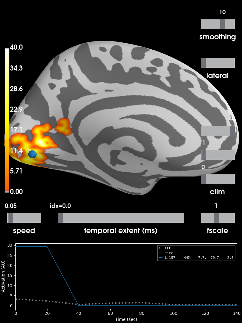
Visualize the clusters
print('Visualizing clusters.')

#    Now let's build a convenient representation of each cluster, where each
#    cluster becomes a "time point" in the SourceEstimate
stc_all_cluster_vis = summarize_clusters_stc(clu, tstep=tstep,
                                             vertices=fsave_vertices,
                                             subject='fsaverage')

#    Let's actually plot the first "time point" in the SourceEstimate, which
#    shows all the clusters, weighted by duration

subjects_dir = op.join(data_path, 'subjects')
# The brighter the color, the stronger the interaction between
# stimulus modality and stimulus location

brain = stc_all_cluster_vis.plot(subjects_dir=subjects_dir, views='lat',
                                 time_label='temporal extent (ms)',
                                 clim=dict(kind='value', lims=[0, 1, 40]))
brain.save_image('cluster-lh.png')
brain.show_view('medial')
Out:
Visualizing clusters.
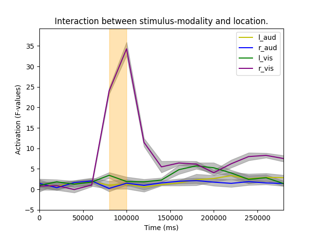
Finally, let’s investigate interaction effect by reconstructing the time courses:
inds_t, inds_v = [(clusters[cluster_ind]) for ii, cluster_ind in
                  enumerate(good_cluster_inds)][0]  # first cluster

times = np.arange(X[0].shape[1]) * tstep * 1e3

plt.figure()
colors = ['y', 'b', 'g', 'purple']
event_ids = ['l_aud', 'r_aud', 'l_vis', 'r_vis']

for ii, (condition, color, eve_id) in enumerate(zip(X, colors, event_ids)):
    # extract time course at cluster vertices
    condition = condition[:, :, inds_v]
    # normally we would normalize values across subjects but
    # here we use data from the same subject so we're good to just
    # create average time series across subjects and vertices.
    mean_tc = condition.mean(axis=2).mean(axis=0)
    std_tc = condition.std(axis=2).std(axis=0)
    plt.plot(times, mean_tc.T, color=color, label=eve_id)
    plt.fill_between(times, mean_tc + std_tc, mean_tc - std_tc, color='gray',
                     alpha=0.5, label='')

ymin, ymax = mean_tc.min() - 5, mean_tc.max() + 5
plt.xlabel('Time (ms)')
plt.ylabel('Activation (F-values)')
plt.xlim(times[[0, -1]])
plt.ylim(ymin, ymax)
plt.fill_betweenx((ymin, ymax), times[inds_t[0]],
                  times[inds_t[-1]], color='orange', alpha=0.3)
plt.legend()
plt.title('Interaction between stimulus-modality and location.')
plt.show()
Total running time of the script: ( 0 minutes 48.056 seconds)
Estimated memory usage: 221 MB