Note
Click here to download the full example code or to run this example in your browser via Binder
07. Save and load T1-weighted MRI scan along with anatomical landmarks in BIDS
When working with MEEG data in the domain of source localization, we usually have to deal with aligning several coordinate systems, such as the coordinate systems of …
the head of a study participant
the recording device (in the case of MEG)
the anatomical MRI scan of a study participant
The process of aligning these frames is also called coregistration, and is
performed with the help of a transformation matrix, called trans in MNE.
In this tutorial, we show how MNE-BIDS can be used to save a T1 weighted
MRI scan in BIDS format, and to encode all information of the trans object
in a BIDS compatible way.
Finally, we will automatically reproduce our trans object from a BIDS
directory.
See the documentation pages in the MNE docs for more information on source alignment and coordinate frames
Note
For this example you will need to install matplotlib and
nilearn on top of your usual mne-bids installation.
# Authors: Stefan Appelhoff <stefan.appelhoff@mailbox.org>
#          Alex Rockhill <aprockhill206@gmail.com>
#          Alex Gramfort <alexandre.gramfort@inria.fr>
# License: BSD (3-clause)
We are importing everything we need for this example:
import os.path as op
import shutil

import numpy as np
import matplotlib.pyplot as plt

import nibabel as nib
from nilearn.plotting import plot_anat

import mne
from mne.datasets import sample
from mne.source_space import head_to_mri

from mne_bids import (write_raw_bids, BIDSPath, write_anat,
                      get_head_mri_trans, print_dir_tree)
We will be using the MNE sample data and write a basic BIDS dataset. For more information, you can checkout the respective example.
data_path = sample.data_path()
event_id = {'Auditory/Left': 1, 'Auditory/Right': 2, 'Visual/Left': 3,
            'Visual/Right': 4, 'Smiley': 5, 'Button': 32}
raw_fname = op.join(data_path, 'MEG', 'sample', 'sample_audvis_raw.fif')
events_data = op.join(data_path, 'MEG', 'sample', 'sample_audvis_raw-eve.fif')
output_path = op.abspath(op.join(data_path, '..', 'MNE-sample-data-bids'))
To ensure the output path doesn’t contain any leftover files from previous tests and example runs, we simply delete it.
Warning
Do not delete directories that may contain important data!
Read the input data and store it as BIDS data.
raw = mne.io.read_raw_fif(raw_fname)
raw.info['line_freq'] = 60  # specify power line frequency as required by BIDS

sub = '01'
ses = '01'
task = 'audiovisual'
run = '01'
bids_path = BIDSPath(subject=sub, session=ses, task=task,
                     run=run, root=output_path)
write_raw_bids(raw, bids_path, events_data=events_data,
               event_id=event_id, overwrite=True)
Out:
Opening raw data file /Users/hoechenberger/mne_data/MNE-sample-data/MEG/sample/sample_audvis_raw.fif...
    Read a total of 3 projection items:
        PCA-v1 (1 x 10²)  idle
        PCA-v2 (1 x 10²)  idle
        PCA-v3 (1 x 10²)  idle
    Range : 25800 ... 192599 =     42.956 ...   320.670 secs
Ready.

Writing '/Users/hoechenberger/mne_data/MNE-sample-data-bids/README'...

References
----------
Appelhoff, S., Sanderson, M., Brooks, T., Vliet, M., Quentin, R., Holdgraf, C., Chaumon, M., Mikulan, E., Tavabi, K., Höchenberger, R., Welke, D., Brunner, C., Rockhill, A., Larson, E., Gramfort, A. and Jas, M. (2019). MNE-BIDS: Organizing electrophysiological data into the BIDS format and facilitating their analysis. Journal of Open Source Software 4: (1896). https://doi.org/10.21105/joss.01896

Niso, G., Gorgolewski, K. J., Bock, E., Brooks, T. L., Flandin, G., Gramfort, A., Henson, R. N., Jas, M., Litvak, V., Moreau, J., Oostenveld, R., Schoffelen, J., Tadel, F., Wexler, J., Baillet, S. (2018). MEG-BIDS, the brain imaging data structure extended to magnetoencephalography. Scientific Data, 5, 180110. https://doi.org/10.1038/sdata.2018.110


Writing '/Users/hoechenberger/mne_data/MNE-sample-data-bids/participants.tsv'...

participant_id  age     sex     hand
sub-01  n/a     n/a     n/a

Writing '/Users/hoechenberger/mne_data/MNE-sample-data-bids/participants.json'...

{
    "participant_id": {
        "Description": "Unique participant identifier"
    },
    "age": {
        "Description": "Age of the participant at time of testing",
        "Units": "years"
    },
    "sex": {
        "Description": "Biological sex of the participant",
        "Levels": {
            "F": "female",
            "M": "male"
        }
    },
    "hand": {
        "Description": "Handedness of the participant",
        "Levels": {
            "R": "right",
            "L": "left",
            "A": "ambidextrous"
        }
    }
}

Writing '/Users/hoechenberger/mne_data/MNE-sample-data-bids/sub-01/ses-01/meg/sub-01_ses-01_coordsystem.json'...

{
    "MEGCoordinateSystem": "ElektaNeuromag",
    "MEGCoordinateUnits": "m",
    "MEGCoordinateSystemDescription": "RAS orientation and the origin between the ears",
    "HeadCoilCoordinates": {
        "NAS": [
            3.725290298461914e-09,
            0.10260561108589172,
            4.190951585769653e-09
        ],
        "LPA": [
            -0.07137660682201385,
            0.0,
            5.122274160385132e-09
        ],
        "RPA": [
            0.07526767998933792,
            0.0,
            5.587935447692871e-09
        ],
        "coil1": [
            0.032922741025686264,
            0.09897983074188232,
            0.07984329760074615
        ],
        "coil2": [
            -0.06998106092214584,
            0.06771647930145264,
            0.06888450682163239
        ],
        "coil3": [
            -0.07260829955339432,
            -0.02086828649044037,
            0.0971473976969719
        ],
        "coil4": [
            0.04996863007545471,
            -0.007233052980154753,
            0.1228904277086258
        ]
    },
    "HeadCoilCoordinateSystem": "ElektaNeuromag",
    "HeadCoilCoordinateUnits": "m"
}

Writing '/Users/hoechenberger/mne_data/MNE-sample-data-bids/sub-01/ses-01/meg/sub-01_ses-01_task-audiovisual_run-01_events.tsv'...

onset   duration        trial_type      value   sample
3.6246181587150867      0.0     Auditory/Right  2       2177
4.237323479067476       0.0     Visual/Left     5       2545
4.946596485779753       0.0     Auditory/Left   1       2971
5.692498614904401       0.0     Visual/Right    6       3419
6.41342634238425        0.0     Auditory/Right  2       3852

Writing '/Users/hoechenberger/mne_data/MNE-sample-data-bids/dataset_description.json'...

{
    "Name": " ",
    "BIDSVersion": "1.4.0",
    "DatasetType": "raw",
    "Authors": [
        "Please cite MNE-BIDS in your publication before removing this (citations in README)"
    ]
}
Reading 0 ... 166799  =      0.000 ...   277.714 secs...

Writing '/Users/hoechenberger/mne_data/MNE-sample-data-bids/sub-01/ses-01/meg/sub-01_ses-01_task-audiovisual_run-01_meg.json'...

{
    "TaskName": "audiovisual",
    "Manufacturer": "Elekta",
    "PowerLineFrequency": 60,
    "SamplingFrequency": 600.614990234375,
    "SoftwareFilters": "n/a",
    "RecordingDuration": 277.7136813300495,
    "RecordingType": "continuous",
    "DewarPosition": "n/a",
    "DigitizedLandmarks": false,
    "DigitizedHeadPoints": false,
    "MEGChannelCount": 306,
    "MEGREFChannelCount": 0,
    "EEGChannelCount": 60,
    "EOGChannelCount": 1,
    "ECGChannelCount": 0,
    "EMGChannelCount": 0,
    "MiscChannelCount": 0,
    "TriggerChannelCount": 9
}

Writing '/Users/hoechenberger/mne_data/MNE-sample-data-bids/sub-01/ses-01/meg/sub-01_ses-01_task-audiovisual_run-01_channels.tsv'...

name    type    units   low_cutoff      high_cutoff     description     sampling_frequency      status  status_description
MEG 0113        MEGGRADPLANAR   T/m     0.10000000149011612     172.17630004882812      Planar Gradiometer      600.614990234375        good    n/a
MEG 0112        MEGGRADPLANAR   T/m     0.10000000149011612     172.17630004882812      Planar Gradiometer      600.614990234375        good    n/a
MEG 0111        MEGMAG  T       0.10000000149011612     172.17630004882812      Magnetometer    600.614990234375        good    n/a
MEG 0122        MEGGRADPLANAR   T/m     0.10000000149011612     172.17630004882812      Planar Gradiometer      600.614990234375        good    n/a
MEG 0123        MEGGRADPLANAR   T/m     0.10000000149011612     172.17630004882812      Planar Gradiometer      600.614990234375        good    n/a
Copying data files to sub-01_ses-01_task-audiovisual_run-01_meg.fif
Reserving possible split file sub-01_ses-01_task-audiovisual_run-01_split-01_meg.fif
Writing /Users/hoechenberger/mne_data/MNE-sample-data-bids/sub-01/ses-01/meg/sub-01_ses-01_task-audiovisual_run-01_meg.fif
Closing /Users/hoechenberger/mne_data/MNE-sample-data-bids/sub-01/ses-01/meg/sub-01_ses-01_task-audiovisual_run-01_meg.fif
[done]

Writing '/Users/hoechenberger/mne_data/MNE-sample-data-bids/sub-01/ses-01/sub-01_ses-01_scans.tsv'...

filename        acq_time
meg/sub-01_ses-01_task-audiovisual_run-01_meg.fif       2002-12-03T19:01:10.720100Z
Wrote /Users/hoechenberger/mne_data/MNE-sample-data-bids/sub-01/ses-01/sub-01_ses-01_scans.tsv entry with meg/sub-01_ses-01_task-audiovisual_run-01_meg.fif.

BIDSPath(
root: /Users/hoechenberger/mne_data/MNE-sample-data-bids
datatype: meg
basename: sub-01_ses-01_task-audiovisual_run-01_meg.fif)
Print the directory tree
Out:
|MNE-sample-data-bids/
|--- README
|--- dataset_description.json
|--- participants.json
|--- participants.tsv
|--- sub-01/
|------ ses-01/
|--------- sub-01_ses-01_scans.tsv
|--------- meg/
|------------ sub-01_ses-01_coordsystem.json
|------------ sub-01_ses-01_task-audiovisual_run-01_channels.tsv
|------------ sub-01_ses-01_task-audiovisual_run-01_events.tsv
|------------ sub-01_ses-01_task-audiovisual_run-01_meg.fif
|------------ sub-01_ses-01_task-audiovisual_run-01_meg.json
Writing T1 image
Now let’s assume that we have also collected some T1 weighted MRI data for
our subject. And furthermore, that we have already aligned our coordinate
frames (using e.g., the coregistration GUI) and obtained a transformation
matrix trans.
# Get the path to our MRI scan
t1_mgh_fname = op.join(data_path, 'subjects', 'sample', 'mri', 'T1.mgz')

# Load the transformation matrix and show what it looks like
trans_fname = op.join(data_path, 'MEG', 'sample',
                      'sample_audvis_raw-trans.fif')
trans = mne.read_trans(trans_fname)
print(trans)
Out:
<Transform | head->MRI (surface RAS)>
[[ 0.99930954  0.01275934  0.0348942   0.00206991]
 [ 0.00998479  0.81240475 -0.58300853  0.01130214]
 [-0.03578702  0.58295429  0.81171638 -0.02755522]
 [ 0.          0.          0.          1.        ]]
We can save the MRI to our existing BIDS directory and at the same time
create a JSON sidecar file that contains metadata, we will later use to
retrieve our transformation matrix trans. The metadata will here
consist of the coordinates of three anatomical landmarks (LPA, Nasion and
RPA (=left and right preauricular points) expressed in voxel coordinates
w.r.t. the T1 image.
# First create the BIDSPath object.
t1w_bids_path = \
    BIDSPath(subject=sub, session=ses, root=output_path, suffix='T1w')

# We use the write_anat function
t1w_bids_path = write_anat(
    image=t1_mgh_fname,  # path to the MRI scan
    bids_path=t1w_bids_path,
    raw=raw,  # the raw MEG data file connected to the MRI
    trans=trans,  # our transformation matrix
    verbose=True  # this will print out the sidecar file
)
anat_dir = t1w_bids_path.directory
Out:
Writing '/Users/hoechenberger/mne_data/MNE-sample-data-bids/sub-01/ses-01/anat/sub-01_ses-01_T1w.json'...

{
    "AnatomicalLandmarkCoordinates": {
        "LPA": [
            197.25741411263368,
            153.0008593581418,
            138.5894600936019
        ],
        "NAS": [
            124.62090614299716,
            95.74083565348268,
            222.65942693440599
        ],
        "RPA": [
            50.71437932937833,
            158.24882153365422,
            140.05367187187042
        ]
    }
}
Let’s have another look at our BIDS directory
Out:
|MNE-sample-data-bids/
|--- README
|--- dataset_description.json
|--- participants.json
|--- participants.tsv
|--- sub-01/
|------ ses-01/
|--------- sub-01_ses-01_scans.tsv
|--------- anat/
|------------ sub-01_ses-01_T1w.json
|------------ sub-01_ses-01_T1w.nii.gz
|--------- meg/
|------------ sub-01_ses-01_coordsystem.json
|------------ sub-01_ses-01_task-audiovisual_run-01_channels.tsv
|------------ sub-01_ses-01_task-audiovisual_run-01_events.tsv
|------------ sub-01_ses-01_task-audiovisual_run-01_meg.fif
|------------ sub-01_ses-01_task-audiovisual_run-01_meg.json
Our BIDS dataset is now ready to be shared. We can easily estimate the
transformation matrix using MNE-BIDS and the BIDS dataset.
Out:
Opening raw data file /Users/hoechenberger/mne_data/MNE-sample-data-bids/sub-01/ses-01/meg/sub-01_ses-01_task-audiovisual_run-01_meg.fif...
    Read a total of 3 projection items:
        PCA-v1 (1 x 10²)  idle
        PCA-v2 (1 x 10²)  idle
        PCA-v3 (1 x 10²)  idle
    Range : 25800 ... 192599 =     42.956 ...   320.670 secs
Ready.
Reading events from /Users/hoechenberger/mne_data/MNE-sample-data-bids/sub-01/ses-01/meg/sub-01_ses-01_task-audiovisual_run-01_events.tsv.
Reading channel info from /Users/hoechenberger/mne_data/MNE-sample-data-bids/sub-01/ses-01/meg/sub-01_ses-01_task-audiovisual_run-01_channels.tsv.
/Users/hoechenberger/Development/mne-bids/mne_bids/read.py:339: RuntimeWarning: The unit for channel(s) STI 001, STI 002, STI 003, STI 004, STI 005, STI 006, STI 014, STI 015, STI 016 has changed from V to NA.
  raw.set_channel_types(channel_type_dict)
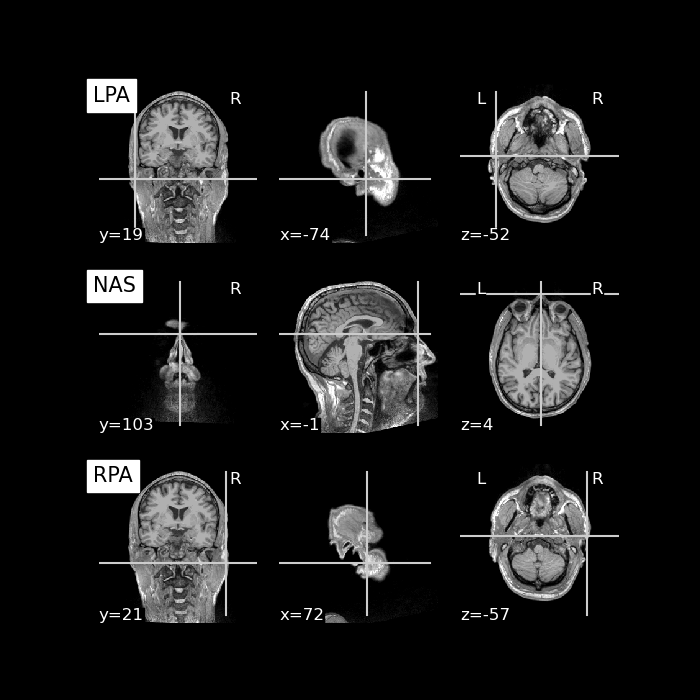
Finally, let’s use the T1 weighted MRI image and plot the anatomical
landmarks Nasion, LPA, and RPA onto the brain image. For that, we can
extract the location of Nasion, LPA, and RPA from the MEG file, apply our
transformation matrix trans, and plot the results.
# Get Landmarks from MEG file, 0, 1, and 2 correspond to LPA, NAS, RPA
# and the 'r' key will provide us with the xyz coordinates. The coordinates
# are expressed here in MEG Head coordinate system.
pos = np.asarray((raw.info['dig'][0]['r'],
                  raw.info['dig'][1]['r'],
                  raw.info['dig'][2]['r']))

# We now use the ``head_to_mri`` function from MNE-Python to convert MEG
# coordinates to MRI scanner RAS space. For the conversion we use our
# estimated transformation matrix and the MEG coordinates extracted from the
# raw file. `subjects` and `subjects_dir` are used internally, to point to
# the T1-weighted MRI file: `t1_mgh_fname`. Coordinates are is mm.
mri_pos = head_to_mri(pos=pos,
                      subject='sample',
                      mri_head_t=estim_trans,
                      subjects_dir=op.join(data_path, 'subjects'))

# Our MRI written to BIDS, we got `anat_dir` from our `write_anat` function
t1_nii_fname = op.join(anat_dir, 'sub-01_ses-01_T1w.nii.gz')

# Plot it
fig, axs = plt.subplots(3, 1, figsize=(7, 7), facecolor='k')
for point_idx, label in enumerate(('LPA', 'NAS', 'RPA')):
    plot_anat(t1_nii_fname, axes=axs[point_idx],
              cut_coords=mri_pos[point_idx, :],
              title=label, vmax=160)
plt.show()
Writing FLASH MRI image
We can write another types of MRI data such as FLASH images for BEM models
flash_mgh_fname = \
    op.join(data_path, 'subjects', 'sample', 'mri', 'flash', 'mef05.mgz')

flash_bids_path = \
    BIDSPath(subject=sub, session=ses, root=output_path, suffix='FLASH')

write_anat(
    image=flash_mgh_fname,
    bids_path=flash_bids_path,
    verbose=True
)
Out:
BIDSPath(
root: /Users/hoechenberger/mne_data/MNE-sample-data-bids
datatype: anat
basename: sub-01_ses-01_FLASH.nii.gz)
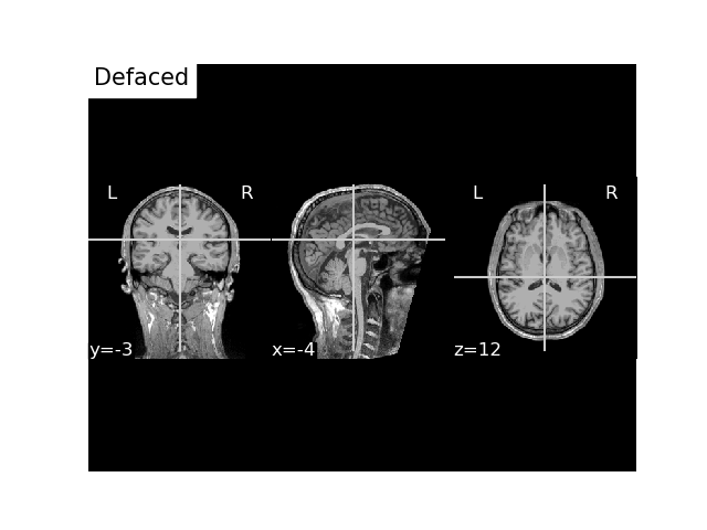
Writing defaced and anonymized T1 image
We can deface the MRI for anonymization by passing deface=True.
t1w_bids_path = write_anat(
    image=t1_mgh_fname,  # path to the MRI scan
    bids_path=bids_path,
    raw=raw,  # the raw MEG data file connected to the MRI
    trans=trans,  # our transformation matrix
    deface=True,
    overwrite=True,
    verbose=True  # this will print out the sidecar file
)
anat_dir = t1w_bids_path.directory

# Our MRI written to BIDS, we got `anat_dir` from our `write_anat` function
t1_nii_fname = op.join(anat_dir, 'sub-01_ses-01_T1w.nii.gz')

# Plot it
fig, ax = plt.subplots()
plot_anat(t1_nii_fname, axes=ax, title='Defaced', vmax=160)
plt.show()
Out:
Writing '/Users/hoechenberger/mne_data/MNE-sample-data-bids/sub-01/ses-01/anat/sub-01_ses-01_T1w.json'...

{
    "AnatomicalLandmarkCoordinates": {
        "LPA": [
            197.25741411263368,
            153.0008593581418,
            138.5894600936019
        ],
        "NAS": [
            124.62090614299716,
            95.74083565348268,
            222.65942693440599
        ],
        "RPA": [
            50.71437932937833,
            158.24882153365422,
            140.05367187187042
        ]
    }
}
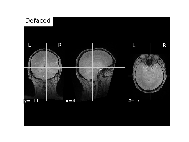
Writing defaced and anonymized FLASH MRI image
Defacing the FLASH is a bit more complicated because it uses different coordinates than the T1. Since, in the example dataset, we used the head surface (which was reconstructed by freesurfer from the T1) to align the digitization points, the points are relative to the T1-defined coordinate system (called surface or TkReg RAS). Thus, you can you can provide the T1 or you can find the fiducials in FLASH voxel space or scanner RAS coordinates using your favorite 3D image view (e.g. freeview). You can also read the fiducial coordinates from the raw and apply the trans yourself. Let’s explore the different options to do this.
Option 1 : Pass t1w with raw and trans
flash_bids_path = write_anat(
    image=flash_mgh_fname,  # path to the MRI scan
    bids_path=flash_bids_path,
    raw=raw,
    trans=trans,
    t1w=t1_mgh_fname,
    deface=True,
    overwrite=True,
    verbose=True  # this will print out the sidecar file
)

# Our MRI written to BIDS, we got `anat_dir` from our `write_anat` function
flash_nii_fname = op.join(anat_dir, 'sub-01_ses-01_FLASH.nii.gz')

# Plot it
fig, ax = plt.subplots()
plot_anat(flash_nii_fname, axes=ax, title='Defaced', vmax=700)
plt.show()

Out:
Writing '/Users/hoechenberger/mne_data/MNE-sample-data-bids/sub-01/ses-01/anat/sub-01_ses-01_FLASH.json'...

{
    "AnatomicalLandmarkCoordinates": {
        "LPA": [
            124.51988917211392,
            156.7554808781791,
            164.5250043352138
        ],
        "NAS": [
            28.620126675736444,
            116.1185261240982,
            95.42797291038784
        ],
        "RPA": [
            120.56940719564132,
            157.75593669628364,
            17.937353558892525
        ]
    }
}
Option 2 : Use manual landmarks coordinates in scanner RAS for FLASH image
You can find such landmarks with a 3D image viewer (e.g. freeview). Note that, in freeview, this is called “RAS” and not “TkReg RAS”
flash_ras_landmarks = \
    np.array([[-74.53102838, 19.62854953, -52.2888194],
              [-1.89454315, 103.69850925, 4.97120376],
              [72.01200673, 21.09274883, -57.53678375]]) / 1e3  # mm -> m

landmarks = mne.channels.make_dig_montage(
    lpa=flash_ras_landmarks[0],
    nasion=flash_ras_landmarks[1],
    rpa=flash_ras_landmarks[2],
    coord_frame='ras'
)

flash_bids_path = write_anat(
    image=flash_mgh_fname,  # path to the MRI scan
    bids_path=flash_bids_path,
    landmarks=landmarks,
    deface=True,
    overwrite=True,
    verbose=True  # this will print out the sidecar file
)

# Plot it
fig, ax = plt.subplots()
plot_anat(flash_nii_fname, axes=ax, title='Defaced', vmax=700)
plt.show()

Out:
Writing '/Users/hoechenberger/mne_data/MNE-sample-data-bids/sub-01/ses-01/anat/sub-01_ses-01_FLASH.json'...

{
    "AnatomicalLandmarkCoordinates": {
        "LPA": [
            124.51988917137612,
            156.75548087980883,
            164.525004336295
        ],
        "NAS": [
            28.62012667241129,
            116.11852612679817,
            95.42797290948731
        ],
        "RPA": [
            120.56940719949279,
            157.75593669708275,
            17.937353558283036
        ]
    }
}
Option 3 : Compute the landmarks in scanner RAS or mri voxel space from trans
Get Landmarks from MEG file, 0, 1, and 2 correspond to LPA, NAS, RPA and the ‘r’ key will provide us with the xyz coordinates.
Note
We can use in the head_to_mri function based on T1 as the T1 and FLASH images are already registered.
head_pos = np.asarray((raw.info['dig'][0]['r'],
                       raw.info['dig'][1]['r'],
                       raw.info['dig'][2]['r']))

ras_pos = head_to_mri(pos=head_pos,
                      subject='sample',
                      mri_head_t=trans,
                      subjects_dir=op.join(data_path, 'subjects')) / 1e3

montage_ras = mne.channels.make_dig_montage(
    lpa=ras_pos[0],
    nasion=ras_pos[1],
    rpa=ras_pos[2],
    coord_frame='ras'
)

# pass FLASH scanner RAS coordinates
flash_bids_path = write_anat(
    image=flash_mgh_fname,  # path to the MRI scan
    bids_path=flash_bids_path,
    landmarks=montage_ras,
    deface=True,
    overwrite=True,
    verbose=True  # this will print out the sidecar file
)

# Plot it
fig, ax = plt.subplots()
plot_anat(flash_nii_fname, axes=ax, title='Defaced', vmax=700)
plt.show()

Out:
Writing '/Users/hoechenberger/mne_data/MNE-sample-data-bids/sub-01/ses-01/anat/sub-01_ses-01_FLASH.json'...

{
    "AnatomicalLandmarkCoordinates": {
        "LPA": [
            124.51988917211392,
            156.75548087817913,
            164.5250043352138
        ],
        "NAS": [
            28.620126675736458,
            116.1185261240982,
            95.42797291038782
        ],
        "RPA": [
            120.56940719564132,
            157.75593669628364,
            17.937353558892525
        ]
    }
}
Let’s now pass it in voxel coordinates
flash_mri_hdr = nib.load(flash_mgh_fname).header
flash_vox_pos = mne.transforms.apply_trans(
    flash_mri_hdr.get_ras2vox(), ras_pos * 1e3)

montage_flash_vox = mne.channels.make_dig_montage(
    lpa=flash_vox_pos[0],
    nasion=flash_vox_pos[1],
    rpa=flash_vox_pos[2],
    coord_frame='mri_voxel'
)

# pass FLASH voxel coordinates
flash_bids_path = write_anat(
    image=flash_mgh_fname,  # path to the MRI scan
    bids_path=flash_bids_path,
    landmarks=montage_flash_vox,
    deface=True,
    overwrite=True,
    verbose=True  # this will print out the sidecar file
)

# Plot it
fig, ax = plt.subplots()
plot_anat(flash_nii_fname, axes=ax, title='Defaced', vmax=700)
plt.show()
Out:
Writing '/Users/hoechenberger/mne_data/MNE-sample-data-bids/sub-01/ses-01/anat/sub-01_ses-01_FLASH.json'...

{
    "AnatomicalLandmarkCoordinates": {
        "LPA": [
            124.51990546203085,
            156.7554883687488,
            164.52500410386176
        ],
        "NAS": [
            28.620148111909458,
            116.11853374996387,
            95.42797273575347
        ],
        "RPA": [
            120.56942384578899,
            157.755944459811,
            17.937353305263002
        ]
    }
}
Total running time of the script: ( 0 minutes 58.945 seconds)