Plotting sensor layouts of MEG systems

Show sensor layouts of different MEG systems.

# Author: Eric Larson <larson.eric.d@gmail.com>
#
# License: BSD (3-clause)

import os.path as op

import mne
from mne.io import read_raw_fif, read_raw_ctf, read_raw_bti, read_raw_kit
from mne.io import read_raw_artemis123
from mne.datasets import sample, spm_face, testing
from mne.viz import plot_alignment, set_3d_title

print(__doc__)

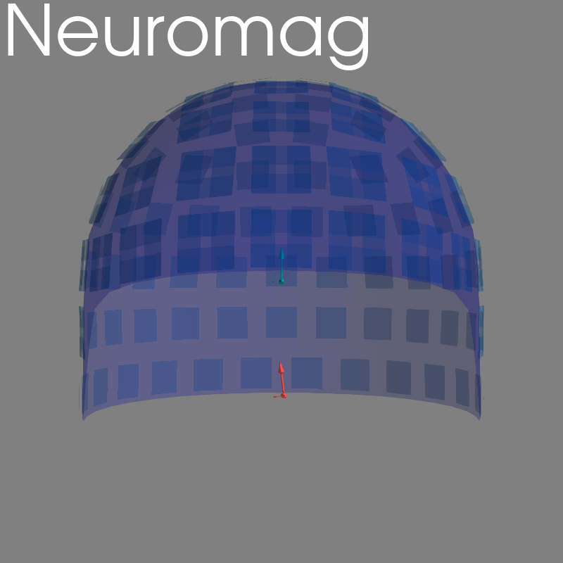
Neuromag

kwargs = dict(eeg=False, coord_frame='meg', show_axes=True, verbose=True)

raw = read_raw_fif(sample.data_path() + '/MEG/sample/sample_audvis_raw.fif')
fig = plot_alignment(raw.info, meg=('helmet', 'sensors'), **kwargs)
set_3d_title(figure=fig, title='Neuromag')

Out:

Opening raw data file /home/circleci/mne_data/MNE-sample-data/MEG/sample/sample_audvis_raw.fif...
    Read a total of 3 projection items:
        PCA-v1 (1 x 102)  idle
        PCA-v2 (1 x 102)  idle
        PCA-v3 (1 x 102)  idle
    Range : 25800 ... 192599 =     42.956 ...   320.670 secs
Ready.
Getting helmet for system 306m

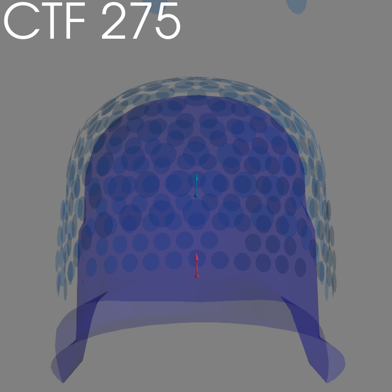
CTF

raw = read_raw_ctf(spm_face.data_path() +
                   '/MEG/spm/SPM_CTF_MEG_example_faces1_3D.ds')
fig = plot_alignment(raw.info, meg=('helmet', 'sensors', 'ref'), **kwargs)
set_3d_title(figure=fig, title='CTF 275')

Out:

ds directory : /home/circleci/mne_data/MNE-spm-face/MEG/spm/SPM_CTF_MEG_example_faces1_3D.ds
    res4 data read.
    hc data read.
    Separate EEG position data file not present.
    Quaternion matching (desired vs. transformed):
      -0.90   72.01    0.00 mm <->   -0.90   72.01   -0.00 mm (orig :  -43.09   61.46 -252.17 mm) diff =    0.000 mm
       0.90  -72.01    0.00 mm <->    0.90  -72.01   -0.00 mm (orig :   53.49  -45.24 -258.02 mm) diff =    0.000 mm
      98.30    0.00    0.00 mm <->   98.30   -0.00    0.00 mm (orig :   78.60   72.16 -241.87 mm) diff =    0.000 mm
    Coordinate transformations established.
    Polhemus data for 3 HPI coils added
    Device coordinate locations for 3 HPI coils added
    Measurement info composed.
Finding samples for /home/circleci/mne_data/MNE-spm-face/MEG/spm/SPM_CTF_MEG_example_faces1_3D.ds/SPM_CTF_MEG_example_faces1_3D.meg4:
    System clock channel is available, checking which samples are valid.
    1 x 324474 = 324474 samples from 340 chs
Current compensation grade : 3
Getting helmet for system CTF_275

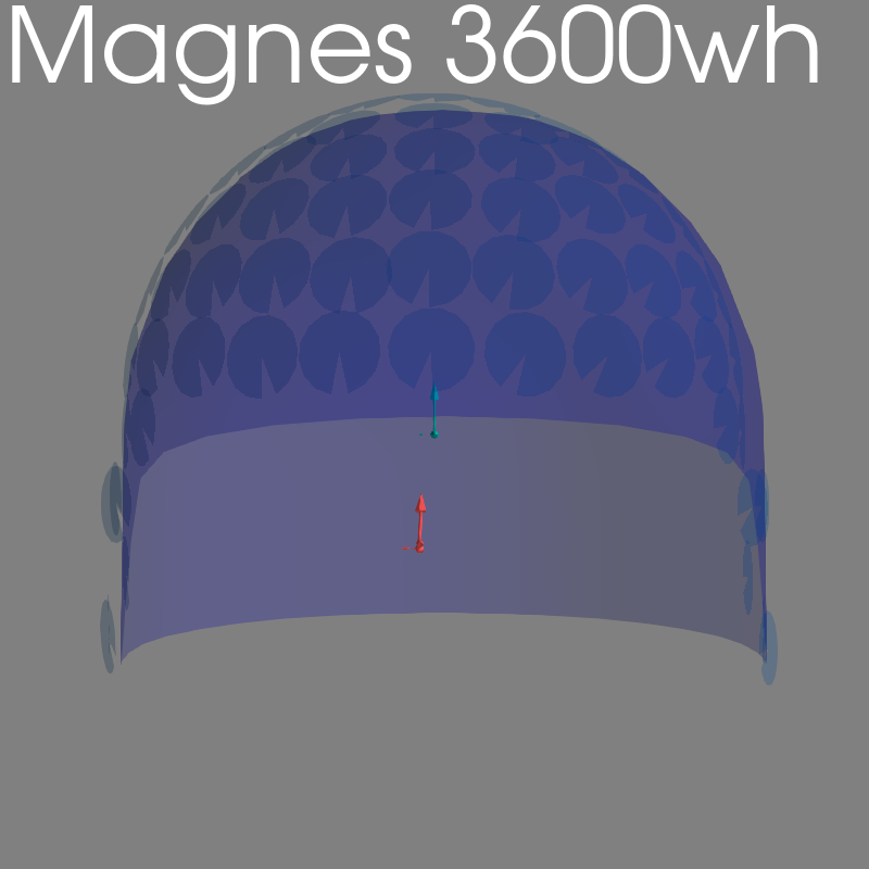
BTi

bti_path = op.abspath(op.dirname(mne.__file__)) + '/io/bti/tests/data/'
raw = read_raw_bti(op.join(bti_path, 'test_pdf_linux'),
                   op.join(bti_path, 'test_config_linux'),
                   op.join(bti_path, 'test_hs_linux'))
fig = plot_alignment(raw.info, meg=('helmet', 'sensors', 'ref'), **kwargs)
set_3d_title(figure=fig, title='Magnes 3600wh')

Out:

Reading 4D PDF file /home/circleci/project/mne/io/bti/tests/data/test_pdf_linux...
Creating Neuromag info structure ...
... Setting channel info structure.
... putting coil transforms in Neuromag coordinates
... Reading digitization points from /home/circleci/project/mne/io/bti/tests/data/test_hs_linux
Currently direct inclusion of 4D weight tables is not supported. For critical use cases please take into account the MNE command "mne_create_comp_data" to include weights as printed out by the 4D "print_table" routine.
Getting helmet for system Magnes_3600wh

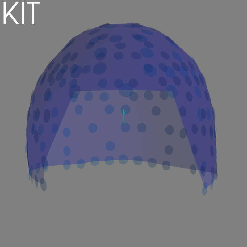
KIT

kit_path = op.abspath(op.dirname(mne.__file__)) + '/io/kit/tests/data/'
raw = read_raw_kit(op.join(kit_path, 'test.sqd'))
fig = plot_alignment(raw.info, meg=('helmet', 'sensors'), **kwargs)
set_3d_title(figure=fig, title='KIT')

Out:

Extracting SQD Parameters from /home/circleci/project/mne/io/kit/tests/data/test.sqd...
Creating Raw.info structure...
Setting channel info structure...
Creating Info structure...
Ready.
Getting helmet for system KIT (derived from 157 MEG channel locations)

Artemis123

raw = read_raw_artemis123(op.join(
    testing.data_path(), 'ARTEMIS123',
    'Artemis_Data_2017-04-14-10h-38m-59s_Phantom_1k_HPI_1s.bin'))
fig = plot_alignment(raw.info, meg=('helmet', 'sensors', 'ref'), **kwargs)
set_3d_title(figure=fig, title='Artemis123')

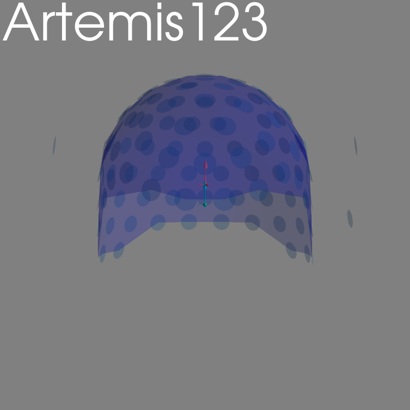
Out:

Reading header...
Loading mne loc file /home/circleci/project/mne/io/artemis123/resources/Artemis123_mneLoc.csv
Using 4 HPI coils: 140 150 160 170 Hz
Line interference frequencies:  Hz
Using time window: 250.0 ms
Fitting 3 HPI coil locations at up to 1 time points (0.3 sec duration)

  0%|          | cHPI amplitudes : 0/1 [00:00<?,       ?it/s]
100%|##########| cHPI amplitudes : 1/1 [00:00<00:00,  255.08it/s]
Computing 1863 HPI location guesses (1 cm grid in a 8.2 cm sphere)
HPIFIT: 3 coils digitized in order 1 2 3
HPI consistency of isotrak and hpifit is OK.

  0%|          | cHPI locations  : 0/1 [00:00<?,       ?it/s]
100%|##########| cHPI locations  : 1/1 [00:00<00:00,   13.23it/s]
100%|##########| cHPI locations  : 1/1 [00:00<00:00,   13.15it/s]
HPI coil 1 - location goodness of fit (0.997)
HPI coil 2 - location goodness of fit (0.999)
HPI coil 3 - location goodness of fit (0.999)
Assuming Cardinal HPIs
Getting helmet for system ARTEMIS123 (derived from 123 MEG channel locations)

Estimated memory usage: 25 MB