The SourceEstimate data structure

Source estimates, commonly referred to as STC (Source Time Courses), are obtained from source localization methods. Source localization method solve the so-called ‘inverse problem’. MNE provides different methods for solving it: dSPM, sLORETA, LCMV, MxNE etc.

Source localization consists in projecting the EEG/MEG sensor data into a 3-dimensional ‘source space’ positioned in the individual subject’s brain anatomy. Hence the data is transformed such that the recorded time series at each sensor location maps to time series at each spatial location of the ‘source space’ where is defined our source estimates.

An STC object contains the amplitudes of the sources over time. It only stores the amplitudes of activations but not the locations of the sources. To get access to the locations you need to have the source space (often abbreviated src) used to compute the forward operator (often abbreviated fwd).

See Head model and forward computation for more details on forward modeling, and Source localization with MNE/dSPM/sLORETA/eLORETA for an example of source localization with dSPM, sLORETA or eLORETA.

Source estimates come in different forms:

• mne.SourceEstimate: For cortically constrained source spaces.

• mne.VolSourceEstimate: For volumetric source spaces

• mne.VectorSourceEstimate: For cortically constrained source spaces with vector-valued source activations (strength and orientation)

• mne.MixedSourceEstimate: For source spaces formed of a combination of cortically constrained and volumetric sources.

Note

(Vector) SourceEstimate are surface representations mostly used together with FreeSurfer surface representations.

Let’s get ourselves an idea of what a mne.SourceEstimate really is. We first set up the environment and load some data:

import os

from mne import read_source_estimate
from mne.datasets import sample

print(__doc__)

# Paths to example data
sample_dir_raw = sample.data_path()
sample_dir = os.path.join(sample_dir_raw, 'MEG', 'sample')
subjects_dir = os.path.join(sample_dir_raw, 'subjects')

fname_stc = os.path.join(sample_dir, 'sample_audvis-meg')

Load and inspect example data

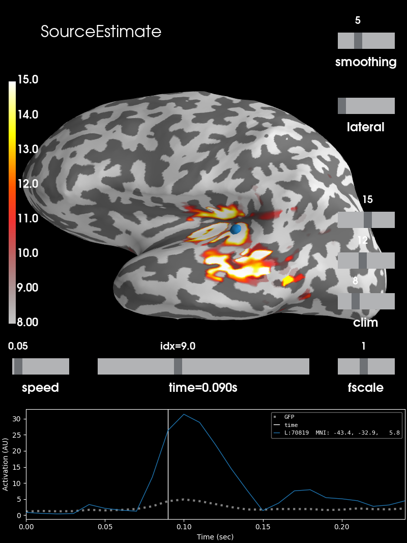
This data set contains source estimation data from an audio visual task. It has been mapped onto the inflated cortical surface representation obtained from FreeSurfer using the dSPM method. It highlights a noticeable peak in the auditory cortices.

Let’s see how it looks like.

stc = read_source_estimate(fname_stc, subject='sample')

# Define plotting parameters
surfer_kwargs = dict(
    hemi='lh', subjects_dir=subjects_dir,
    clim=dict(kind='value', lims=[8, 12, 15]), views='lateral',
    initial_time=0.09, time_unit='s', size=(800, 800),
    smoothing_steps=5)

# Plot surface
brain = stc.plot(**surfer_kwargs)

# Add title
brain.add_text(0.1, 0.9, 'SourceEstimate', 'title', font_size=16)

SourceEstimate (stc)

A source estimate contains the time series of a activations at spatial locations defined by the source space. In the context of a FreeSurfer surfaces - which consist of 3D triangulations - we could call each data point on the inflated brain representation a vertex . If every vertex represents the spatial location of a time series, the time series and spatial location can be written into a matrix, where to each vertex (rows) at multiple time points (columns) a value can be assigned. This value is the strength of our signal at a given point in space and time. Exactly this matrix is stored in stc.data.

Let’s have a look at the shape

shape = stc.data.shape

print('The data has %s vertex locations with %s sample points each.' % shape)

Out:

The data has 7498 vertex locations with 25 sample points each.

We see that stc carries 7498 time series of 25 samples length. Those time series belong to 7498 vertices, which in turn represent locations on the cortical surface. So where do those vertex values come from?

FreeSurfer separates both hemispheres and creates surfaces representation for left and right hemisphere. Indices to surface locations are stored in stc.vertices. This is a list with two arrays of integers, that index a particular vertex of the FreeSurfer mesh. A value of 42 would hence map to the x,y,z coordinates of the mesh with index 42. See next section on how to get access to the positions in a mne.SourceSpaces object.

Since both hemispheres are always represented separately, both attributes introduced above, can also be obtained by selecting the respective hemisphere. This is done by adding the correct prefix (lh or rh).

shape_lh = stc.lh_data.shape

print('The left hemisphere has %s vertex locations with %s sample points each.'
      % shape_lh)

Out:

The left hemisphere has 3732 vertex locations with 25 sample points each.

Since we did not change the time representation, only the selected subset of vertices and hence only the row size of the matrix changed. We can check if the rows of stc.lh_data and stc.rh_data sum up to the value we had before.

is_equal = stc.lh_data.shape[0] + stc.rh_data.shape[0] == stc.data.shape[0]

print('The number of vertices in stc.lh_data and stc.rh_data do ' +
      ('not ' if not is_equal else '') +
      'sum up to the number of rows in stc.data')

Out:

The number of vertices in stc.lh_data and stc.rh_data do sum up to the number of rows in stc.data

Indeed and as the mindful reader already suspected, the same can be said about vertices. stc.lh_vertno thereby maps to the left and stc.rh_vertno to the right inflated surface representation of FreeSurfer.

Relationship to SourceSpaces (src)

As mentioned above, src carries the mapping from stc to the surface. The surface is built up from a triangulated mesh for each hemisphere. Each triangle building up a face consists of 3 vertices. Since src is a list of two source spaces (left and right hemisphere), we can access the respective data by selecting the source space first. Faces building up the left hemisphere can be accessed via src[0]['tris'], where the index \(0\) stands for the left and \(1\) for the right hemisphere.

The values in src[0][‘tris’] refer to row indices in src[0]['rr']. Here we find the actual coordinates of the surface mesh. Hence every index value for vertices will select a coordinate from here. Furthermore src[0]['vertno'] stores the same data as stc.lh_vertno, except when working with sparse solvers such as mne.inverse_sparse.mixed_norm(), as then only a fraction of vertices actually have non-zero activations.

In other words stc.lh_vertno equals src[0]['vertno'], whereas stc.rh_vertno equals src[1]['vertno']. Thus the Nth time series in stc.lh_data corresponds to the Nth value in stc.lh_vertno and src[0][‘vertno’] respectively, which in turn map the time series to a specific location on the surface, represented as the set of cartesian coordinates stc.lh_vertno[N] in src[0]['rr'].

Let’s obtain the peak amplitude of the data as vertex and time point index

peak_vertex, peak_time = stc.get_peak(hemi='lh', vert_as_index=True,
                                      time_as_index=True)

The first value thereby indicates which vertex and the second which time point index from within stc.lh_vertno or stc.lh_data is used. We can use the respective information to get the index of the surface vertex resembling the peak and its value.

peak_vertex_surf = stc.lh_vertno[peak_vertex]

peak_value = stc.lh_data[peak_vertex, peak_time]

Let’s visualize this as well, using the same surfer_kwargs as in the beginning.

brain = stc.plot(**surfer_kwargs)

# We add the new peak coordinate (as vertex index) as an annotation dot
brain.add_foci(peak_vertex_surf, coords_as_verts=True, hemi='lh', color='blue')

# We add a title as well, stating the amplitude at this time and location
brain.add_text(0.1, 0.9, 'Peak coordinate', 'title', font_size=14)

Summary

stc is a class of MNE-Python, representing the transformed time series obtained from source estimation. For both hemispheres the data is stored separately in stc.lh_data and stc.rh_data in form of a \(m \times n\) matrix, where \(m\) is the number of spatial locations belonging to that hemisphere and \(n\) the number of time points.

stc.lh_vertno and stc.rh_vertno correspond to src[0]['vertno'] and src[1]['vertno']. Those are the indices of locations on the surface representation.

The surface’s mesh coordinates are stored in src[0]['rr'] and src[1]['rr'] for left and right hemisphere. 3D coordinates can be accessed by the above logic:

>>> lh_coordinates = src[0]['rr'][stc.lh_vertno]
>>> lh_data = stc.lh_data

or:

>>> rh_coordinates = src[1]['rr'][src[1]['vertno']]
>>> rh_data = stc.rh_data

Estimated memory usage: 64 MB