Compute multivariate measures of the imaginary part of coherency

This example demonstrates how multivariate methods based on the imaginary part of coherency [1] can be used to compute connectivity between whole sets of sensors, and how spatial patterns of this connectivity can be interpreted.

The methods in question are: the maximised imaginary part of coherency (MIC); and the multivariate interaction measure (MIM; as well as its extension, the global interaction measure, GIM).

# Author: Thomas S. Binns <t.s.binns@outlook.com>
# License: BSD (3-clause)

import numpy as np
from matplotlib import pyplot as plt
from matplotlib import patheffects as pe

import mne
from mne import EvokedArray, make_fixed_length_epochs
from mne.datasets.fieldtrip_cmc import data_path
from mne_connectivity import seed_target_indices, spectral_connectivity_epochs

Background

Multivariate forms of signal analysis allow you to simultaneously consider the activity of multiple signals. In the case of connectivity, the interaction between multiple sensors can be analysed at once, producing a single connectivity spectrum. This approach brings not only practical benefits (e.g. easier interpretability of results from the dimensionality reduction), but can also offer methodological improvements (e.g. enhanced signal-to-noise ratio and reduced bias).

A popular bivariate measure of connectivity is the imaginary part of coherency, which looks at the correlation between two signals in the frequency domain and is immune to spurious connectivity arising from volume conduction artefacts [2]. However, depending on the degree of source mixing, this measure is susceptible to biased estimates of connectivity based on the spatial proximity of sensors [1].

To overcome this limitation, spatial filters can be used to estimate connectivity free from this source mixing-dependent bias, which additionally increases the signal-to-noise ratio and allows signals to be analysed in a multivariate manner [1]. This approach leads to the following methods: the maximised imaginary part of coherency (MIC); and the multivariate interaction measure (MIM).

We start by loading some example MEG data and dividing it into two-second-long epochs.

raw = mne.io.read_raw_ctf(data_path() / "SubjectCMC.ds")
raw.pick("mag")
raw.crop(50.0, 110.0).load_data()
raw.notch_filter(50)
raw.resample(100)

epochs = make_fixed_length_epochs(raw, duration=2.0).load_data()

ds directory : /home/circleci/mne_data/MNE-fieldtrip_cmc-data/SubjectCMC.ds
    res4 data read.
    hc data read.
    Separate EEG position data file not present.
    Quaternion matching (desired vs. transformed):
       0.33   78.32    0.00 mm <->    0.33   78.32    0.00 mm (orig :  -71.62   40.46 -256.48 mm) diff =    0.000 mm
      -0.33  -78.32   -0.00 mm <->   -0.33  -78.32   -0.00 mm (orig :   39.27  -70.16 -258.60 mm) diff =    0.000 mm
     114.65    0.00   -0.00 mm <->  114.65    0.00   -0.00 mm (orig :   64.35   66.64 -262.01 mm) diff =    0.000 mm
    Coordinate transformations established.
    Polhemus data for 3 HPI coils added
    Device coordinate locations for 3 HPI coils added
Picked positions of 4 EEG channels from channel info
    4 EEG locations added to Polhemus data.
    Measurement info composed.
Finding samples for /home/circleci/mne_data/MNE-fieldtrip_cmc-data/SubjectCMC.ds/SubjectCMC.meg4:
    System clock channel is available, checking which samples are valid.
    75 x 12000 = 911610 samples from 191 chs
    390 samples omitted at the end
Current compensation grade : 0
Removing 5 compensators from info because not all compensation channels were picked.
Reading 0 ... 72000  =      0.000 ...    60.000 secs...
Filtering raw data in 1 contiguous segment
Setting up band-stop filter from 49 - 51 Hz

FIR filter parameters
---------------------
Designing a one-pass, zero-phase, non-causal bandstop filter:
- Windowed time-domain design (firwin) method
- Hamming window with 0.0194 passband ripple and 53 dB stopband attenuation
- Lower passband edge: 49.38
- Lower transition bandwidth: 0.50 Hz (-6 dB cutoff frequency: 49.12 Hz)
- Upper passband edge: 50.62 Hz
- Upper transition bandwidth: 0.50 Hz (-6 dB cutoff frequency: 50.88 Hz)
- Filter length: 7921 samples (6.601 s)

[Parallel(n_jobs=1)]: Done  17 tasks      | elapsed:    0.1s
[Parallel(n_jobs=1)]: Done  71 tasks      | elapsed:    0.2s
Not setting metadata
30 matching events found
No baseline correction applied
0 projection items activated
Using data from preloaded Raw for 30 events and 200 original time points ...
0 bad epochs dropped

We will focus on connectivity between sensors over the left and right hemispheres, with 75 sensors in the left hemisphere designated as seeds, and 76 sensors in the right hemisphere designated as targets.

# left hemisphere sensors
seeds = [idx for idx, ch_info in enumerate(epochs.info["chs"]) if ch_info["loc"][0] < 0]
# right hemisphere sensors
targets = [
    idx for idx, ch_info in enumerate(epochs.info["chs"]) if ch_info["loc"][0] > 0
]

multivar_indices = (np.array([seeds]), np.array([targets]))

seed_names = [epochs.info["ch_names"][idx] for idx in seeds]
target_names = [epochs.info["ch_names"][idx] for idx in targets]

# multivariate imaginary part of coherency
(mic, mim) = spectral_connectivity_epochs(
    epochs, method=["mic", "mim"], indices=multivar_indices, fmin=5, fmax=30, rank=None
)

# bivariate imaginary part of coherency (for comparison)
bivar_indices = seed_target_indices(seeds, targets)
imcoh = spectral_connectivity_epochs(
    epochs, method="imcoh", indices=bivar_indices, fmin=5, fmax=30
)

Adding metadata with 3 columns
Connectivity computation...
    computing connectivity for 1 connections
    using t=0.000s..1.990s for estimation (200 points)
    frequencies: 5.0Hz..30.0Hz (51 points)
Estimated data ranks:
    connection 1 - seeds (75); targets (76)
    Using multitaper spectrum estimation with 7 DPSS windows
    the following metrics will be computed: MIC, MIM
    computing cross-spectral density for epoch 1
    computing cross-spectral density for epoch 2
    computing cross-spectral density for epoch 3
    computing cross-spectral density for epoch 4
    computing cross-spectral density for epoch 5
    computing cross-spectral density for epoch 6
    computing cross-spectral density for epoch 7
    computing cross-spectral density for epoch 8
    computing cross-spectral density for epoch 9
    computing cross-spectral density for epoch 10
    computing cross-spectral density for epoch 11
    computing cross-spectral density for epoch 12
    computing cross-spectral density for epoch 13
    computing cross-spectral density for epoch 14
    computing cross-spectral density for epoch 15
    computing cross-spectral density for epoch 16
    computing cross-spectral density for epoch 17
    computing cross-spectral density for epoch 18
    computing cross-spectral density for epoch 19
    computing cross-spectral density for epoch 20
    computing cross-spectral density for epoch 21
    computing cross-spectral density for epoch 22
    computing cross-spectral density for epoch 23
    computing cross-spectral density for epoch 24
    computing cross-spectral density for epoch 25
    computing cross-spectral density for epoch 26
    computing cross-spectral density for epoch 27
    computing cross-spectral density for epoch 28
    computing cross-spectral density for epoch 29
    computing cross-spectral density for epoch 30
Computing MIC for connection 1 of 1

  0%|          | frequency blocks : 0/51 [00:00<?,       ?it/s]
  2%|▏         | frequency blocks : 1/51 [00:00<00:00,   50.37it/s]
  4%|▍         | frequency blocks : 2/51 [00:00<00:00,   53.28it/s]
  6%|▌         | frequency blocks : 3/51 [00:00<00:01,   39.04it/s]
  8%|▊         | frequency blocks : 4/51 [00:00<00:01,   42.57it/s]
 10%|▉         | frequency blocks : 5/51 [00:00<00:01,   44.99it/s]
 12%|█▏        | frequency blocks : 6/51 [00:00<00:01,   33.51it/s]
 14%|█▎        | frequency blocks : 7/51 [00:00<00:01,   35.87it/s]
 16%|█▌        | frequency blocks : 8/51 [00:00<00:01,   37.95it/s]
 18%|█▊        | frequency blocks : 9/51 [00:00<00:01,   32.69it/s]
 20%|█▉        | frequency blocks : 10/51 [00:00<00:01,   34.50it/s]
 22%|██▏       | frequency blocks : 11/51 [00:00<00:01,   36.16it/s]
 24%|██▎       | frequency blocks : 12/51 [00:00<00:01,   31.77it/s]
 25%|██▌       | frequency blocks : 13/51 [00:00<00:01,   33.24it/s]
 27%|██▋       | frequency blocks : 14/51 [00:00<00:01,   34.63it/s]
 29%|██▉       | frequency blocks : 15/51 [00:00<00:01,   31.26it/s]
 31%|███▏      | frequency blocks : 16/51 [00:00<00:01,   32.53it/s]
 33%|███▎      | frequency blocks : 17/51 [00:00<00:01,   33.75it/s]
 35%|███▌      | frequency blocks : 18/51 [00:00<00:00,   34.89it/s]
 37%|███▋      | frequency blocks : 19/51 [00:00<00:00,   32.24it/s]
 39%|███▉      | frequency blocks : 20/51 [00:00<00:00,   33.36it/s]
 41%|████      | frequency blocks : 21/51 [00:00<00:00,   34.42it/s]
 43%|████▎     | frequency blocks : 22/51 [00:00<00:00,   31.66it/s]
 45%|████▌     | frequency blocks : 23/51 [00:00<00:00,   32.67it/s]
 47%|████▋     | frequency blocks : 24/51 [00:00<00:00,   33.66it/s]
 49%|████▉     | frequency blocks : 25/51 [00:00<00:00,   31.58it/s]
 51%|█████     | frequency blocks : 26/51 [00:00<00:00,   32.54it/s]
 53%|█████▎    | frequency blocks : 27/51 [00:00<00:00,   33.47it/s]
 55%|█████▍    | frequency blocks : 28/51 [00:00<00:00,   31.28it/s]
 57%|█████▋    | frequency blocks : 29/51 [00:00<00:00,   32.16it/s]
 59%|█████▉    | frequency blocks : 30/51 [00:00<00:00,   33.06it/s]
 61%|██████    | frequency blocks : 31/51 [00:00<00:00,   31.03it/s]
 63%|██████▎   | frequency blocks : 32/51 [00:00<00:00,   31.89it/s]
 65%|██████▍   | frequency blocks : 33/51 [00:00<00:00,   32.75it/s]
 67%|██████▋   | frequency blocks : 34/51 [00:01<00:00,   33.61it/s]
 69%|██████▊   | frequency blocks : 35/51 [00:01<00:00,   31.60it/s]
 71%|███████   | frequency blocks : 36/51 [00:01<00:00,   32.43it/s]
 73%|███████▎  | frequency blocks : 37/51 [00:01<00:00,   33.24it/s]
 75%|███████▍  | frequency blocks : 38/51 [00:01<00:00,   31.27it/s]
 76%|███████▋  | frequency blocks : 39/51 [00:01<00:00,   32.08it/s]
 78%|███████▊  | frequency blocks : 40/51 [00:01<00:00,   32.84it/s]
 80%|████████  | frequency blocks : 41/51 [00:01<00:00,   30.99it/s]
 82%|████████▏ | frequency blocks : 42/51 [00:01<00:00,   31.78it/s]
 84%|████████▍ | frequency blocks : 43/51 [00:01<00:00,   32.55it/s]
 86%|████████▋ | frequency blocks : 44/51 [00:01<00:00,   30.78it/s]
 88%|████████▊ | frequency blocks : 45/51 [00:01<00:00,   31.56it/s]
 90%|█████████ | frequency blocks : 46/51 [00:01<00:00,   29.56it/s]
 92%|█████████▏| frequency blocks : 47/51 [00:01<00:00,   30.31it/s]
 94%|█████████▍| frequency blocks : 48/51 [00:01<00:00,   31.09it/s]
 96%|█████████▌| frequency blocks : 49/51 [00:01<00:00,   31.85it/s]
 98%|█████████▊| frequency blocks : 50/51 [00:01<00:00,   30.44it/s]
100%|██████████| frequency blocks : 51/51 [00:01<00:00,   31.18it/s]
100%|██████████| frequency blocks : 51/51 [00:01<00:00,   31.98it/s]
Computing MIM for connection 1 of 1

  0%|          | frequency blocks : 0/51 [00:00<?,       ?it/s]
  2%|▏         | frequency blocks : 1/51 [00:00<00:00,   54.75it/s]
  4%|▍         | frequency blocks : 2/51 [00:00<00:00,   54.89it/s]
  6%|▌         | frequency blocks : 3/51 [00:00<00:00,   55.16it/s]
  8%|▊         | frequency blocks : 4/51 [00:00<00:01,   35.92it/s]
 10%|▉         | frequency blocks : 5/51 [00:00<00:01,   38.96it/s]
 12%|█▏        | frequency blocks : 6/51 [00:00<00:01,   40.13it/s]
 14%|█▎        | frequency blocks : 7/51 [00:00<00:01,   29.76it/s]
 16%|█▌        | frequency blocks : 8/51 [00:00<00:01,   31.96it/s]
 18%|█▊        | frequency blocks : 9/51 [00:00<00:01,   28.15it/s]
 20%|█▉        | frequency blocks : 10/51 [00:00<00:01,   30.01it/s]
 22%|██▏       | frequency blocks : 11/51 [00:00<00:01,   31.72it/s]
 24%|██▎       | frequency blocks : 12/51 [00:00<00:01,   29.08it/s]
 25%|██▌       | frequency blocks : 13/51 [00:00<00:01,   30.58it/s]
 27%|██▋       | frequency blocks : 14/51 [00:00<00:01,   32.02it/s]
 29%|██▉       | frequency blocks : 15/51 [00:00<00:01,   29.25it/s]
 31%|███▏      | frequency blocks : 16/51 [00:00<00:01,   30.53it/s]
 33%|███▎      | frequency blocks : 17/51 [00:00<00:01,   31.77it/s]
 35%|███▌      | frequency blocks : 18/51 [00:00<00:01,   29.39it/s]
 37%|███▋      | frequency blocks : 19/51 [00:00<00:01,   30.53it/s]
 39%|███▉      | frequency blocks : 20/51 [00:00<00:00,   31.66it/s]
 41%|████      | frequency blocks : 21/51 [00:00<00:00,   32.78it/s]
 43%|████▎     | frequency blocks : 22/51 [00:00<00:00,   30.72it/s]
 45%|████▌     | frequency blocks : 23/51 [00:00<00:00,   31.79it/s]
 47%|████▋     | frequency blocks : 24/51 [00:00<00:00,   32.81it/s]
 49%|████▉     | frequency blocks : 25/51 [00:00<00:00,   30.59it/s]
 51%|█████     | frequency blocks : 26/51 [00:00<00:00,   31.58it/s]
 53%|█████▎    | frequency blocks : 27/51 [00:00<00:00,   32.55it/s]
 55%|█████▍    | frequency blocks : 28/51 [00:00<00:00,   30.71it/s]
 57%|█████▋    | frequency blocks : 29/51 [00:00<00:00,   30.99it/s]
 59%|█████▉    | frequency blocks : 30/51 [00:00<00:00,   28.74it/s]
 61%|██████    | frequency blocks : 31/51 [00:01<00:00,   29.34it/s]
 63%|██████▎   | frequency blocks : 32/51 [00:01<00:00,   30.21it/s]
 65%|██████▍   | frequency blocks : 33/51 [00:01<00:00,   28.87it/s]
 67%|██████▋   | frequency blocks : 34/51 [00:01<00:00,   29.75it/s]
 69%|██████▊   | frequency blocks : 35/51 [00:01<00:00,   30.59it/s]
 71%|███████   | frequency blocks : 36/51 [00:01<00:00,   28.99it/s]
 73%|███████▎  | frequency blocks : 37/51 [00:01<00:00,   29.84it/s]
 75%|███████▍  | frequency blocks : 38/51 [00:01<00:00,   30.69it/s]
 76%|███████▋  | frequency blocks : 39/51 [00:01<00:00,   31.53it/s]
 78%|███████▊  | frequency blocks : 40/51 [00:01<00:00,   30.08it/s]
 80%|████████  | frequency blocks : 41/51 [00:01<00:00,   30.90it/s]
 82%|████████▏ | frequency blocks : 42/51 [00:01<00:00,   31.71it/s]
 84%|████████▍ | frequency blocks : 43/51 [00:01<00:00,   30.07it/s]
 86%|████████▋ | frequency blocks : 44/51 [00:01<00:00,   30.88it/s]
 88%|████████▊ | frequency blocks : 45/51 [00:01<00:00,   31.68it/s]
 90%|█████████ | frequency blocks : 46/51 [00:01<00:00,   30.29it/s]
 92%|█████████▏| frequency blocks : 47/51 [00:01<00:00,   31.08it/s]
 94%|█████████▍| frequency blocks : 48/51 [00:01<00:00,   31.85it/s]
 96%|█████████▌| frequency blocks : 49/51 [00:01<00:00,   30.23it/s]
 98%|█████████▊| frequency blocks : 50/51 [00:01<00:00,   31.00it/s]
100%|██████████| frequency blocks : 51/51 [00:01<00:00,   31.74it/s]
100%|██████████| frequency blocks : 51/51 [00:01<00:00,   31.20it/s]
[Connectivity computation done]
Replacing existing metadata with 3 columns
Connectivity computation...
    computing connectivity for 5700 connections
    using t=0.000s..1.990s for estimation (200 points)
    frequencies: 5.0Hz..30.0Hz (51 points)
    Using multitaper spectrum estimation with 7 DPSS windows
    the following metrics will be computed: Imaginary Coherence
    computing cross-spectral density for epoch 1
    computing cross-spectral density for epoch 2
    computing cross-spectral density for epoch 3
    computing cross-spectral density for epoch 4
    computing cross-spectral density for epoch 5
    computing cross-spectral density for epoch 6
    computing cross-spectral density for epoch 7
    computing cross-spectral density for epoch 8
    computing cross-spectral density for epoch 9
    computing cross-spectral density for epoch 10
    computing cross-spectral density for epoch 11
    computing cross-spectral density for epoch 12
    computing cross-spectral density for epoch 13
    computing cross-spectral density for epoch 14
    computing cross-spectral density for epoch 15
    computing cross-spectral density for epoch 16
    computing cross-spectral density for epoch 17
    computing cross-spectral density for epoch 18
    computing cross-spectral density for epoch 19
    computing cross-spectral density for epoch 20
    computing cross-spectral density for epoch 21
    computing cross-spectral density for epoch 22
    computing cross-spectral density for epoch 23
    computing cross-spectral density for epoch 24
    computing cross-spectral density for epoch 25
    computing cross-spectral density for epoch 26
    computing cross-spectral density for epoch 27
    computing cross-spectral density for epoch 28
    computing cross-spectral density for epoch 29
    computing cross-spectral density for epoch 30
[Connectivity computation done]

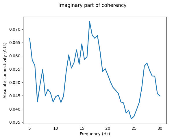
By averaging across each connection between the seeds and targets, we can see that the bivariate measure of the imaginary part of coherency estimates a strong peak in connectivity between seeds and targets around 13-18 Hz, with a weaker peak around 27 Hz.

fig, axis = plt.subplots(1, 1)
axis.plot(imcoh.freqs, np.mean(np.abs(imcoh.get_data()), axis=0), linewidth=2)
axis.set_xlabel("Frequency (Hz)")
axis.set_ylabel("Absolute connectivity (A.U.)")
fig.suptitle("Imaginary part of coherency")

Text(0.5, 0.98, 'Imaginary part of coherency')

Maximised imaginary part of coherency (MIC)

For MIC, a set of spatial filters are found that will maximise the estimated connectivity between the seed and target signals. These maximising filters correspond to the eigenvectors with the largest eigenvalue, derived from an eigendecomposition of information from the cross-spectral density (Eq. 7 of [1]):

\(MIC=\frac{\boldsymbol{\alpha}^T \boldsymbol{E \beta}}{\parallel \boldsymbol{\alpha}\parallel \parallel\boldsymbol{\beta}\parallel}\),

where \(\boldsymbol{\alpha}\) and \(\boldsymbol{\beta}\) are the spatial filters for the seeds and targets, respectively, and \(\boldsymbol{E}\) is the imaginary part of the transformed cross-spectral density between the seeds and targets. All elements are frequency-dependent, however this is omitted for readability. MIC is bound between \([-1, 1]\) where the absolute value reflects connectivity strength and the sign reflects the phase angle difference between signals.

MIC can also be computed between identical sets of seeds and targets, allowing connectivity within a single set of signals to be estimated. This is possible as a result of the exclusion of zero phase lag components from the connectivity estimates, which would otherwise return a perfect correlation.

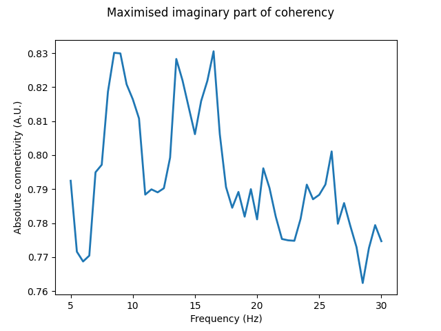
In this instance, we see MIC reveal that in addition to the 13-18 Hz peak, a previously unobserved peak in connectivity around 9 Hz is present. Furthermore, the previous peak around 27 Hz is much less pronounced. This may indicate that the connectivity was the result of some distal interaction exacerbated by strong source mixing, which biased the bivariate connectivity estimate.

fig, axis = plt.subplots(1, 1)
axis.plot(mic.freqs, np.abs(mic.get_data()[0]), linewidth=2)
axis.set_xlabel("Frequency (Hz)")
axis.set_ylabel("Absolute connectivity (A.U.)")
fig.suptitle("Maximised imaginary part of coherency")

Text(0.5, 0.98, 'Maximised imaginary part of coherency')

Furthermore, spatial patterns of connectivity can be constructed from the spatial filters to give a picture of the location of the sources involved in the connectivity. This information is stored under attrs['patterns'] of the connectivity class, with one value per frequency for each channel in the seeds and targets. As with MIC, the absolute value of the patterns reflect the strength, however the sign differences can be used to visualise the orientation of the underlying dipole sources. The spatial patterns are not bound between \([-1, 1]\).

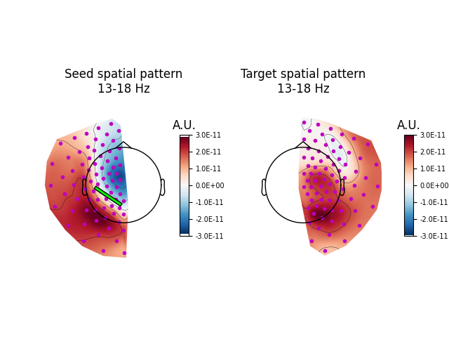
Here, we average across the patterns in the 13-18 Hz range. Plotting the patterns shows that the greatest connectivity between the left and right hemispheres occurs at the left and right posterior and left central regions, based on the areas with the largest absolute values. Using the signs of the values, we can infer the existence of a dipole source between the central and posterior regions of the left hemisphere accounting for the connectivity contributions (represented on the plot as a green line).

# compute average of patterns in desired frequency range
fband = [13, 18]
fband_idx = [mic.freqs.index(freq) for freq in fband]

# patterns have shape [seeds/targets x cons x channels x freqs (x times)]
patterns = np.array(mic.attrs["patterns"])
seed_pattern = patterns[0, :, : len(seeds)]
target_pattern = patterns[1, :, : len(targets)]
# average across frequencies
seed_pattern = np.mean(seed_pattern[0, :, fband_idx[0] : fband_idx[1] + 1], axis=1)
target_pattern = np.mean(target_pattern[0, :, fband_idx[0] : fband_idx[1] + 1], axis=1)

# store the patterns for plotting
seed_info = epochs.copy().pick(seed_names).info
target_info = epochs.copy().pick(target_names).info
seed_pattern = EvokedArray(seed_pattern[:, np.newaxis], seed_info)
target_pattern = EvokedArray(target_pattern[:, np.newaxis], target_info)

# plot the patterns
fig, axes = plt.subplots(1, 4)
seed_pattern.plot_topomap(
    times=0,
    sensors="m.",
    units=dict(mag="A.U."),
    cbar_fmt="%.1E",
    axes=axes[0:2],
    time_format="",
    show=False,
)
target_pattern.plot_topomap(
    times=0,
    sensors="m.",
    units=dict(mag="A.U."),
    cbar_fmt="%.1E",
    axes=axes[2:],
    time_format="",
    show=False,
)
axes[0].set_position((0.1, 0.1, 0.35, 0.7))
axes[1].set_position((0.4, 0.3, 0.02, 0.3))
axes[2].set_position((0.5, 0.1, 0.35, 0.7))
axes[3].set_position((0.9, 0.3, 0.02, 0.3))
axes[0].set_title("Seed spatial pattern\n13-18 Hz")
axes[2].set_title("Target spatial pattern\n13-18 Hz")

# plot the left hemisphere dipole example
axes[0].plot(
    [-0.01, -0.07],
    [-0.07, -0.03],
    color="lime",
    linewidth=2,
    path_effects=[pe.Stroke(linewidth=4, foreground="k"), pe.Normal()],
)

plt.show()

Multivariate interaction measure (MIM)

Although it can be useful to analyse the single, largest connectivity component with MIC, multiple such components exist and can be examined with MIM. MIM can be thought of as an average of all connectivity components between the seeds and targets, and can be useful for an exploration of all available components. It is unnecessary to use the spatial filters of each component explicitly, and instead the desired result can be achieved from \(E\) alone (Eq. 14 of [1]):

\(MIM=tr(\boldsymbol{EE}^T)\),

where again the frequency dependence is omitted. Unlike MIC, MIM is positive-valued and can be > 1. Without normalisation, MIM can be thought of as reflecting the total interaction between the seeds and targets. MIM can be normalised to lie in the range \([0, 1]\) by dividing the scores by the number of unique channels in the seeds and targets. Normalised MIM represents the interaction per channel, which can be biased by factors such as the presence of channels with little to no interaction. In line with the preferences of the method’s authors [1], since normalisation alters the interpretability of the results, normalisation is not performed by default.

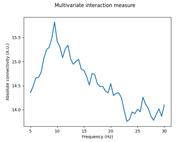
Here we see MIM reveal the strongest connectivity component to be around 10 Hz, with the higher frequency 13-18 Hz connectivity no longer being so prominent. This suggests that, across all components in the data, there may be more lower frequency connectivity sources than higher frequency sources. Thus, when combining these different components in MIM, the peak around 10 Hz remains, but the 13-18 Hz connectivity is diminished relative to the single, largest connectivity component of MIC.

Looking at the values for normalised MIM, we see it has a maximum of ~0.1. The relatively small connectivity values thus indicate that many of the channels show little to no interaction.

fig, axis = plt.subplots(1, 1)
axis.plot(mim.freqs, mim.get_data()[0], linewidth=2)
axis.set_xlabel("Frequency (Hz)")
axis.set_ylabel("Absolute connectivity (A.U.)")
fig.suptitle("Multivariate interaction measure")

n_channels = len(seeds) + len(targets)
normalised_mim = mim.get_data()[0] / n_channels
print(f"Normalised MIM has a maximum value of {normalised_mim.max():.2f}")

Normalised MIM has a maximum value of 0.10

Additionally, the instance where the seeds and targets are identical can be considered as a special case of MIM: the global interaction measure (GIM; Eq. 15 of [1]). Again, this allows connectivity within a single set of signals to be estimated. Computing GIM follows from Eq. 14, however since each interaction is considered twice, correcting the connectivity by a factor of \(\frac{1}{2}\) is necessary (the correction is performed automatically in this implementation). Like MIM, GIM can also be > 1, but it can again be normalised to lie in the range \([0, 1]\) by dividing by the number of unique channels in the seeds and targets. However, since normalisation alters the interpretability of the results (i.e. interaction per channel for normalised GIM vs. total interaction for standard GIM), GIM is not normalised by default.

With GIM, we find a broad connectivity peak around 10 Hz, with an additional peak around 20 Hz. The differences observed with GIM highlight the presence of interactions within each hemisphere that are absent for MIC or MIM. Furthermore, the values for normalised GIM are higher than for MIM, with a maximum of ~0.2, again indicating the presence of interactions across channels within each hemisphere.

indices = (np.array([[*seeds, *targets]]), np.array([[*seeds, *targets]]))
gim = spectral_connectivity_epochs(
    epochs, method="mim", indices=indices, fmin=5, fmax=30, rank=None, verbose=False
)

fig, axis = plt.subplots(1, 1)
axis.plot(gim.freqs, gim.get_data()[0], linewidth=2)
axis.set_xlabel("Frequency (Hz)")
axis.set_ylabel("Connectivity (A.U.)")
fig.suptitle("Global interaction measure")

n_channels = len(seeds) + len(targets)
normalised_gim = gim.get_data()[0] / n_channels
print(f"Normalised GIM has a maximum value of {normalised_gim.max():.2f}")

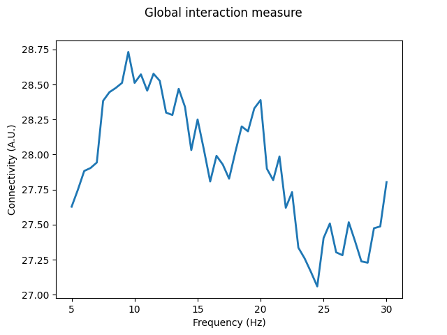
Normalised GIM has a maximum value of 0.19

Handling high-dimensional data

An important issue to consider when using these multivariate methods is overfitting, which risks biasing connectivity estimates to maximise noise in the data. This risk can be reduced by performing a preliminary dimensionality reduction prior to estimating the connectivity with a singular value decomposition (Eqs. 32 & 33 of [1]). The degree of this dimensionality reduction can be specified using the rank argument, which by default will not perform any dimensionality reduction (assuming your data is full rank; see below if not). Choosing an expected rank of the data requires a priori knowledge about the number of components you expect to observe in the data.

When comparing MIC/MIM scores across recordings, it is highly recommended to estimate connectivity from the same number of channels (or equally from the same degree of rank subspace projection) to avoid biases in connectivity estimates. Bias can be avoided by specifying a consistent rank subspace to project to using the rank argument, standardising your connectivity estimates regardless of changes in e.g. the number of channels across recordings. Note that this does not refer to the number of seeds and targets within a connection being identical, rather to the number of seeds and targets across connections.

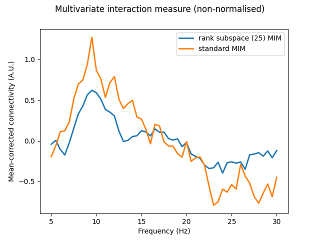
Here, we will project our seed and target data to only the first 25 components of our rank subspace. Results for MIM show that the general spectral pattern of connectivity is retained in the rank subspace-projected data, suggesting that a fair degree of redundant connectivity information is contained in the remaining 50 components of the seed and target data. We also assert that the spatial patterns of MIC are returned in the original sensor space despite this rank subspace projection, being reconstructed using the products of the singular value decomposition (Eqs. 46 & 47 of [1]).

(mic_red, mim_red) = spectral_connectivity_epochs(
    epochs,
    method=["mic", "mim"],
    indices=multivar_indices,
    fmin=5,
    fmax=30,
    rank=([25], [25]),
)

# subtract mean of scores for comparison
mim_red_meansub = mim_red.get_data()[0] - mim_red.get_data()[0].mean()
mim_meansub = mim.get_data()[0] - mim.get_data()[0].mean()

# compare standard and rank subspace-projected MIM
fig, axis = plt.subplots(1, 1)
axis.plot(mim_red.freqs, mim_red_meansub, linewidth=2, label="rank subspace (25) MIM")
axis.plot(mim.freqs, mim_meansub, linewidth=2, label="standard MIM")
axis.set_xlabel("Frequency (Hz)")
axis.set_ylabel("Mean-corrected connectivity (A.U.)")
axis.legend()
fig.suptitle("Multivariate interaction measure (non-normalised)")

# no. channels equal with and without projecting to rank subspace for patterns
assert patterns[0, 0].shape[0] == np.array(mic_red.attrs["patterns"])[0, 0].shape[0]
assert patterns[1, 0].shape[0] == np.array(mic_red.attrs["patterns"])[1, 0].shape[0]

Replacing existing metadata with 3 columns
Connectivity computation...
    computing connectivity for 1 connections
    using t=0.000s..1.990s for estimation (200 points)
    frequencies: 5.0Hz..30.0Hz (51 points)
    Using multitaper spectrum estimation with 7 DPSS windows
    the following metrics will be computed: MIC, MIM
    computing cross-spectral density for epoch 1
    computing cross-spectral density for epoch 2
    computing cross-spectral density for epoch 3
    computing cross-spectral density for epoch 4
    computing cross-spectral density for epoch 5
    computing cross-spectral density for epoch 6
    computing cross-spectral density for epoch 7
    computing cross-spectral density for epoch 8
    computing cross-spectral density for epoch 9
    computing cross-spectral density for epoch 10
    computing cross-spectral density for epoch 11
    computing cross-spectral density for epoch 12
    computing cross-spectral density for epoch 13
    computing cross-spectral density for epoch 14
    computing cross-spectral density for epoch 15
    computing cross-spectral density for epoch 16
    computing cross-spectral density for epoch 17
    computing cross-spectral density for epoch 18
    computing cross-spectral density for epoch 19
    computing cross-spectral density for epoch 20
    computing cross-spectral density for epoch 21
    computing cross-spectral density for epoch 22
    computing cross-spectral density for epoch 23
    computing cross-spectral density for epoch 24
    computing cross-spectral density for epoch 25
    computing cross-spectral density for epoch 26
    computing cross-spectral density for epoch 27
    computing cross-spectral density for epoch 28
    computing cross-spectral density for epoch 29
    computing cross-spectral density for epoch 30
Computing MIC for connection 1 of 1

  0%|          | frequency blocks : 0/51 [00:00<?,       ?it/s]
  6%|▌         | frequency blocks : 3/51 [00:00<00:00,  146.29it/s]
 12%|█▏        | frequency blocks : 6/51 [00:00<00:00,  146.53it/s]
 18%|█▊        | frequency blocks : 9/51 [00:00<00:00,   88.56it/s]
 24%|██▎       | frequency blocks : 12/51 [00:00<00:00,   98.06it/s]
 29%|██▉       | frequency blocks : 15/51 [00:00<00:00,  104.82it/s]
 33%|███▎      | frequency blocks : 17/51 [00:00<00:00,   82.91it/s]
 39%|███▉      | frequency blocks : 20/51 [00:00<00:00,   89.61it/s]
 45%|████▌     | frequency blocks : 23/51 [00:00<00:00,   95.13it/s]
 49%|████▉     | frequency blocks : 25/51 [00:00<00:00,   80.98it/s]
 55%|█████▍    | frequency blocks : 28/51 [00:00<00:00,   85.53it/s]
 61%|██████    | frequency blocks : 31/51 [00:00<00:00,   90.07it/s]
 65%|██████▍   | frequency blocks : 33/51 [00:00<00:00,   79.69it/s]
 71%|███████   | frequency blocks : 36/51 [00:00<00:00,   84.02it/s]
 76%|███████▋  | frequency blocks : 39/51 [00:00<00:00,   88.02it/s]
 80%|████████  | frequency blocks : 41/51 [00:00<00:00,   79.57it/s]
 86%|████████▋ | frequency blocks : 44/51 [00:00<00:00,   83.24it/s]
 92%|█████████▏| frequency blocks : 47/51 [00:00<00:00,   86.72it/s]
 96%|█████████▌| frequency blocks : 49/51 [00:00<00:00,   79.18it/s]
100%|██████████| frequency blocks : 51/51 [00:00<00:00,   83.09it/s]
Computing MIM for connection 1 of 1

  0%|          | frequency blocks : 0/51 [00:00<?,       ?it/s]
  6%|▌         | frequency blocks : 3/51 [00:00<00:00,  146.83it/s]
 12%|█▏        | frequency blocks : 6/51 [00:00<00:00,  147.31it/s]
 14%|█▎        | frequency blocks : 7/51 [00:00<00:00,   85.27it/s]
 20%|█▉        | frequency blocks : 10/51 [00:00<00:00,   98.42it/s]
 25%|██▌       | frequency blocks : 13/51 [00:00<00:00,  107.66it/s]
 29%|██▉       | frequency blocks : 15/51 [00:00<00:00,   81.31it/s]
 35%|███▌      | frequency blocks : 18/51 [00:00<00:00,   88.90it/s]
 41%|████      | frequency blocks : 21/51 [00:00<00:00,   94.92it/s]
 45%|████▌     | frequency blocks : 23/51 [00:00<00:00,   79.90it/s]
 49%|████▉     | frequency blocks : 25/51 [00:00<00:00,   82.57it/s]
 53%|█████▎    | frequency blocks : 27/51 [00:00<00:00,   85.06it/s]
 57%|█████▋    | frequency blocks : 29/51 [00:00<00:00,   87.44it/s]
 59%|█████▉    | frequency blocks : 30/51 [00:00<00:00,   74.86it/s]
 65%|██████▍   | frequency blocks : 33/51 [00:00<00:00,   79.13it/s]
 71%|███████   | frequency blocks : 36/51 [00:00<00:00,   83.12it/s]
 73%|███████▎  | frequency blocks : 37/51 [00:00<00:00,   73.69it/s]
 78%|███████▊  | frequency blocks : 40/51 [00:00<00:00,   77.84it/s]
 84%|████████▍ | frequency blocks : 43/51 [00:00<00:00,   81.51it/s]
 88%|████████▊ | frequency blocks : 45/51 [00:00<00:00,   74.09it/s]
 94%|█████████▍| frequency blocks : 48/51 [00:00<00:00,   77.84it/s]
100%|██████████| frequency blocks : 51/51 [00:00<00:00,   81.42it/s]
100%|██████████| frequency blocks : 51/51 [00:00<00:00,   81.75it/s]
[Connectivity computation done]

In the case that your data is not full rank and rank is left as None, an automatic rank computation is performed and an appropriate degree of dimensionality reduction will be enforced. The rank of the data is determined by computing the singular values of the data and finding those within a factor of \(1e^{-6}\) relative to the largest singular value.

Whilst unlikely, there may be scenarios in which this threshold may be too lenient. In these cases, you should inspect the singular values of your data to identify an appropriate degree of dimensionality reduction to perform, which you can then specify manually using the rank argument. The code below shows one possible approach for finding an appropriate rank of close-to-singular data with a more conservative threshold.

# gets the singular values of the data
s = np.linalg.svd(raw.get_data(), compute_uv=False)
# finds how many singular values are 'close' to the largest singular value
rank = np.count_nonzero(s >= s[0] * 1e-4)  # 1e-4 is the 'closeness' criteria

Limitations

These multivariate methods offer many benefits in the form of dimensionality reduction, signal-to-noise ratio improvements, and invariance to estimate-biasing source mixing; however, no method is perfect. The immunity of the imaginary part of coherency to volume conduction comes from the fact that these artefacts have zero phase lag, and hence a zero-valued imaginary component. By projecting the complex-valued coherency to the imaginary axis, signals of a given magnitude with phase lag differences close to 90° or 270° see their contributions to the connectivity estimate increased relative to comparable signals with phase lag differences close to 0° or 180°. Therefore, the imaginary part of coherency is biased towards connectivity involving 90° and 270° phase lag difference components.

Whilst this is not a limitation specific to the multivariate extension of this measure, these multivariate methods can introduce further bias: when maximising the imaginary part of coherency, components with phase lag differences close to 90° and 270° will likely give higher connectivity estimates, and so may be prioritised by the spatial filters.

Such a limitation should be kept in mind when estimating connectivity using these methods. Possible sanity checks can involve comparing the spectral profiles of MIC/MIM to coherence and the imaginary part of coherency computed on the same data, as well as comparing to other multivariate measures, such as canonical coherence [3].

References

[1] (1,2,3,4,5,6,7,8,9)

Arne Ewald, Laura Marzetti, Filippo Zappasodi, Frank C. Meinecke, and Guido Nolte. Estimating true brain connectivity from EEG/MEG data invariant to linear and static transformations in sensor space. NeuroImage, 60(1):476–488, 2012. doi:10.1016/j.neuroimage.2011.11.084.

[2]

Guido Nolte, Ou Bai, Lewis Wheaton, Zoltan Mari, Sherry Vorbach, and Mark Hallett. Identifying true brain interaction from EEG data using the imaginary part of coherency. Clinical Neurophysiology, 115(10):2292–2307, 2004. doi:10.1016/j.clinph.2004.04.029.

[3]

Carmen Vidaurre, Guido Nolte, Ingmar E.J. de Vries, M. Gómez, Tjeerd W. Boonstra, K.-R. Müller, Arno Villringer, and Vadim V. Nikulin. Canonical maximization of coherence: a novel tool for investigation of neuronal interactions between two datasets. NeuroImage, 201:116009, 2019. doi:10.1016/j.neuroimage.2019.116009.