Note

Click here to download the full example code

Brainstorm Elekta phantom dataset tutorial¶

Here we compute the evoked from raw for the Brainstorm Elekta phantom tutorial dataset. For comparison, see 1 and:

https://neuroimage.usc.edu/brainstorm/Tutorials/PhantomElekta

References¶

1: Tadel F, Baillet S, Mosher JC, Pantazis D, Leahy RM. Brainstorm: A User-Friendly Application for MEG/EEG Analysis. Computational Intelligence and Neuroscience, vol. 2011, Article ID 879716, 13 pages, 2011. doi:10.1155/2011/879716

# Authors: Eric Larson <larson.eric.d@gmail.com>
#
# License: BSD (3-clause)

import os.path as op
import numpy as np
import matplotlib.pyplot as plt

import mne
from mne import find_events, fit_dipole
from mne.datasets.brainstorm import bst_phantom_elekta
from mne.io import read_raw_fif

print(__doc__)

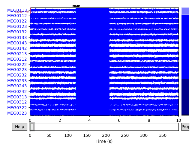
The data were collected with an Elekta Neuromag VectorView system at 1000 Hz and low-pass filtered at 330 Hz. Here the medium-amplitude (200 nAm) data are read to construct instances of mne.io.Raw.

data_path = bst_phantom_elekta.data_path(verbose=True)
subject = 'sample'

raw_fname = op.join(data_path, 'kojak_all_200nAm_pp_no_chpi_no_ms_raw.fif')
raw = read_raw_fif(raw_fname)

Out:

Opening raw data file /home/circleci/mne_data/MNE-brainstorm-data/bst_phantom_elekta/kojak_all_200nAm_pp_no_chpi_no_ms_raw.fif...
    Read a total of 13 projection items:
        planar-0.0-115.0-PCA-01 (1 x 306)  idle
        planar-0.0-115.0-PCA-02 (1 x 306)  idle
        planar-0.0-115.0-PCA-03 (1 x 306)  idle
        planar-0.0-115.0-PCA-04 (1 x 306)  idle
        planar-0.0-115.0-PCA-05 (1 x 306)  idle
        axial-0.0-115.0-PCA-01 (1 x 306)  idle
        axial-0.0-115.0-PCA-02 (1 x 306)  idle
        axial-0.0-115.0-PCA-03 (1 x 306)  idle
        axial-0.0-115.0-PCA-04 (1 x 306)  idle
        axial-0.0-115.0-PCA-05 (1 x 306)  idle
        axial-0.0-115.0-PCA-06 (1 x 306)  idle
        axial-0.0-115.0-PCA-07 (1 x 306)  idle
        axial-0.0-115.0-PCA-08 (1 x 306)  idle
    Range : 47000 ... 437999 =     47.000 ...   437.999 secs
Ready.

Data channel array consisted of 204 MEG planor gradiometers, 102 axial magnetometers, and 3 stimulus channels. Let’s get the events for the phantom, where each dipole (1-32) gets its own event:

events = find_events(raw, 'STI201')
raw.plot(events=events)
raw.info['bads'] = ['MEG1933', 'MEG2421']

Out:

events found
Event IDs: [   1    2    3    4    5    6    7    8    9   10   11   12   13   14
 16   17   18   19   20   21   22   23   24   25   26   27   28
 30   31   32  256  768 1792 3840 7936]

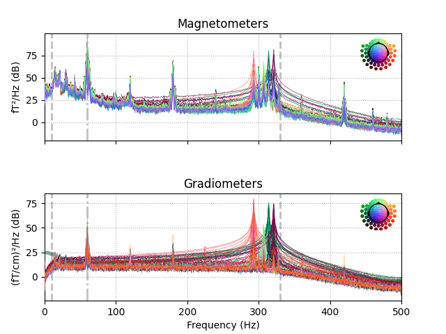
The data have strong line frequency (60 Hz and harmonics) and cHPI coil noise (five peaks around 300 Hz). Here we plot only out to 60 seconds to save memory:

raw.plot_psd(tmax=30., average=False)

Out:

Effective window size : 2.048 (s)
Effective window size : 2.048 (s)

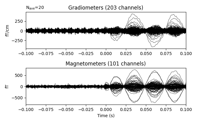
Our phantom produces sinusoidal bursts at 20 Hz:

raw.plot(events=events)

Now we epoch our data, average it, and look at the first dipole response. The first peak appears around 3 ms. Because we low-passed at 40 Hz, we can also decimate our data to save memory.

tmin, tmax = -0.1, 0.1
bmax = -0.05  # Avoid capture filter ringing into baseline
event_id = list(range(1, 33))
epochs = mne.Epochs(raw, events, event_id, tmin, tmax, baseline=(None, bmax),
                    preload=False)
epochs['1'].average().plot(time_unit='s')

Gradiometers (203 channels), Magnetometers (101 channels)

Out:

Not setting metadata
Not setting metadata
640 matching events found
Applying baseline correction (mode: mean)
Created an SSP operator (subspace dimension = 13)
13 projection items activated

Let’s use a sphere head geometry model and let’s see the coordinate alignment and the sphere location. The phantom is properly modeled by a single-shell sphere with origin (0., 0., 0.).

sphere = mne.make_sphere_model(r0=(0., 0., 0.), head_radius=0.08)

mne.viz.plot_alignment(epochs.info, subject=subject, show_axes=True,
                       bem=sphere, dig=True, surfaces='inner_skull')

Out:

Equiv. model fitting -> RV = 0.00372821 %
mu1 = 0.943946    lambda1 = 0.139079
mu2 = 0.665521    lambda2 = 0.684839
mu3 = -0.0973038    lambda3 = -0.013548
Set up EEG sphere model with scalp radius    80.0 mm

    Triangle neighbors and vertex normals...
Getting helmet for system 306m

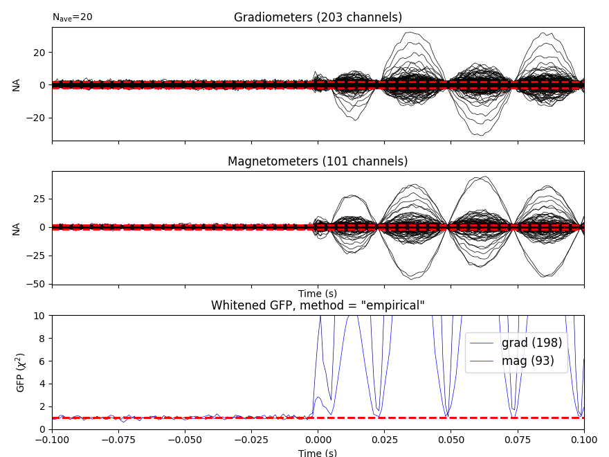
Let’s do some dipole fits. We first compute the noise covariance, then do the fits for each event_id taking the time instant that maximizes the global field power.

# here we can get away with using method='oas' for speed (faster than "shrunk")
# but in general "shrunk" is usually better
cov = mne.compute_covariance(epochs, tmax=bmax)
mne.viz.plot_evoked_white(epochs['1'].average(), cov)

data = []
t_peak = 0.036  # true for Elekta phantom
for ii in event_id:
    # Avoid the first and last trials -- can contain dipole-switching artifacts
    evoked = epochs[str(ii)][1:-1].average().crop(t_peak, t_peak)
    data.append(evoked.data[:, 0])
evoked = mne.EvokedArray(np.array(data).T, evoked.info, tmin=0.)
del epochs
dip, residual = fit_dipole(evoked, cov, sphere, n_jobs=1)

Gradiometers (203 channels), Magnetometers (101 channels), Whitened GFP, method = "empirical"

Out:

Loading data for 20 events and 201 original time points ...
0 bad epochs dropped
Loading data for 20 events and 201 original time points ...
0 bad epochs dropped
Loading data for 20 events and 201 original time points ...
0 bad epochs dropped
Loading data for 20 events and 201 original time points ...
0 bad epochs dropped
Loading data for 20 events and 201 original time points ...
0 bad epochs dropped
Loading data for 20 events and 201 original time points ...
0 bad epochs dropped
Loading data for 20 events and 201 original time points ...
0 bad epochs dropped
Loading data for 20 events and 201 original time points ...
0 bad epochs dropped
Loading data for 20 events and 201 original time points ...
0 bad epochs dropped
Loading data for 20 events and 201 original time points ...
0 bad epochs dropped
Loading data for 20 events and 201 original time points ...
0 bad epochs dropped
Loading data for 20 events and 201 original time points ...
0 bad epochs dropped
Loading data for 20 events and 201 original time points ...
0 bad epochs dropped
Loading data for 20 events and 201 original time points ...
0 bad epochs dropped
Loading data for 20 events and 201 original time points ...
0 bad epochs dropped
Loading data for 20 events and 201 original time points ...
0 bad epochs dropped
Loading data for 20 events and 201 original time points ...
0 bad epochs dropped
Loading data for 20 events and 201 original time points ...
0 bad epochs dropped
Loading data for 20 events and 201 original time points ...
0 bad epochs dropped
Loading data for 20 events and 201 original time points ...
0 bad epochs dropped
Loading data for 20 events and 201 original time points ...
0 bad epochs dropped
Loading data for 20 events and 201 original time points ...
0 bad epochs dropped
Loading data for 20 events and 201 original time points ...
0 bad epochs dropped
Loading data for 20 events and 201 original time points ...
0 bad epochs dropped
Loading data for 20 events and 201 original time points ...
0 bad epochs dropped
Loading data for 20 events and 201 original time points ...
0 bad epochs dropped
Loading data for 20 events and 201 original time points ...
0 bad epochs dropped
Loading data for 20 events and 201 original time points ...
0 bad epochs dropped
Loading data for 20 events and 201 original time points ...
0 bad epochs dropped
Loading data for 20 events and 201 original time points ...
0 bad epochs dropped
Loading data for 20 events and 201 original time points ...
0 bad epochs dropped
Loading data for 20 events and 201 original time points ...
0 bad epochs dropped
Computing rank from data with rank=None
    Using tolerance 3.8e-08 (2.2e-16 eps * 304 dim * 5.7e+05  max singular value)
    Estimated rank (mag + grad): 291
    MEG: rank 291 computed from 304 data channels with 13 projectors
    Created an SSP operator (subspace dimension = 13)
    Setting small MEG eigenvalues to zero (without PCA)
Reducing data rank from 304 -> 291
Estimating covariance using EMPIRICAL
Done.
Number of samples used : 32640
[done]
Computing rank from covariance with rank=None
    Using tolerance 3.8e-11 (2.2e-16 eps * 203 dim * 8.4e+02  max singular value)
    Estimated rank (grad): 198
    GRAD: rank 198 computed from 203 data channels with 5 projectors
Computing rank from covariance with rank=None
    Using tolerance 3.4e-14 (2.2e-16 eps * 101 dim * 1.5  max singular value)
    Estimated rank (mag): 93
    MAG: rank 93 computed from 101 data channels with 8 projectors
    Created an SSP operator (subspace dimension = 13)
Computing rank from covariance with rank={'grad': 198, 'mag': 93, 'meg': 291}
    Setting small MEG eigenvalues to zero (without PCA)
    Created the whitener using a noise covariance matrix with rank 291 (13 small eigenvalues omitted)
BEM               : <ConductorModel | Sphere (3 layers): r0=[0.0, 0.0, 0.0] R=80 mm>
MRI transform     : identity
Sphere model      : origin at (   0.00    0.00    0.00) mm, rad =    0.1 mm
Guess grid        :   20.0 mm
Guess mindist     :    5.0 mm
Guess exclude     :   20.0 mm
Using standard MEG coil definitions.

Coordinate transformation: MRI (surface RAS) -> head
     1.000000  0.000000  0.000000       0.00 mm
     0.000000  1.000000  0.000000       0.00 mm
     0.000000  0.000000  1.000000       0.00 mm
     0.000000  0.000000  0.000000       1.00
Coordinate transformation: MEG device -> head
     0.976295 -0.211976  0.043756       0.29 mm
     0.206488  0.972764  0.105326       0.57 mm
    -0.064891 -0.093794  0.993475       5.41 mm
     0.000000  0.000000  0.000000       1.00
2 bad channels total
Read 304 MEG channels from info
99 coil definitions read
Coordinate transformation: MEG device -> head
     0.976295 -0.211976  0.043756       0.29 mm
     0.206488  0.972764  0.105326       0.57 mm
    -0.064891 -0.093794  0.993475       5.41 mm
     0.000000  0.000000  0.000000       1.00
MEG coil definitions created in head coordinates.
Decomposing the sensor noise covariance matrix...
    Created an SSP operator (subspace dimension = 13)
Computing rank from covariance with rank=None
    Using tolerance 5.7e-11 (2.2e-16 eps * 304 dim * 8.4e+02  max singular value)
    Estimated rank (mag + grad): 291
    MEG: rank 291 computed from 304 data channels with 13 projectors
    Setting small MEG eigenvalues to zero (without PCA)
    Created the whitener using a noise covariance matrix with rank 291 (13 small eigenvalues omitted)

---- Computing the forward solution for the guesses...
Making a spherical guess space with radius    72.0 mm...
Filtering (grid =     20 mm)...
Surface CM = (   0.0    0.0    0.0) mm
Surface fits inside a sphere with radius   72.0 mm
Surface extent:
    x =  -72.0 ...   72.0 mm
    y =  -72.0 ...   72.0 mm
    z =  -72.0 ...   72.0 mm
Grid extent:
    x =  -80.0 ...   80.0 mm
    y =  -80.0 ...   80.0 mm
    z =  -80.0 ...   80.0 mm
729 sources before omitting any.
178 sources after omitting infeasible sources not within 20.0 - 72.0 mm.
170 sources remaining after excluding the sources outside the surface and less than    5.0 mm inside.
Go through all guess source locations...
[done 170 sources]
---- Fitted :     0.0 ms
---- Fitted :     1.0 ms
---- Fitted :     2.0 ms
---- Fitted :     3.0 ms
---- Fitted :     4.0 ms
---- Fitted :     5.0 ms
---- Fitted :     6.0 ms
---- Fitted :     7.0 ms
---- Fitted :     8.0 ms
---- Fitted :     9.0 ms
---- Fitted :    10.0 ms
---- Fitted :    11.0 ms
---- Fitted :    12.0 ms
---- Fitted :    13.0 ms
---- Fitted :    14.0 ms
---- Fitted :    15.0 ms
---- Fitted :    16.0 ms
---- Fitted :    17.0 ms
---- Fitted :    18.0 ms
---- Fitted :    19.0 ms
---- Fitted :    20.0 ms
---- Fitted :    21.0 ms
---- Fitted :    22.0 ms
---- Fitted :    23.0 ms
---- Fitted :    24.0 ms
---- Fitted :    25.0 ms
---- Fitted :    26.0 ms
---- Fitted :    27.0 ms
---- Fitted :    28.0 ms
---- Fitted :    29.0 ms
---- Fitted :    30.0 ms
---- Fitted :    31.0 ms
Projections have already been applied. Setting proj attribute to True.
32 time points fitted

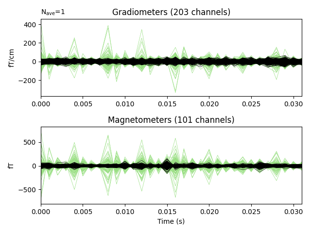
Do a quick visualization of how much variance we explained, putting the data and residuals on the same scale (here the “time points” are the 32 dipole peak values that we fit):

fig, axes = plt.subplots(2, 1)
evoked.plot(axes=axes)
for ax in axes:
    ax.texts = []
    for line in ax.lines:
        line.set_color('#98df81')
residual.plot(axes=axes)

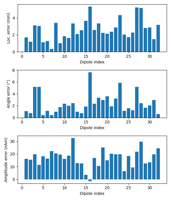
Now we can compare to the actual locations, taking the difference in mm:

actual_pos, actual_ori = mne.dipole.get_phantom_dipoles()
actual_amp = 100.  # nAm

fig, (ax1, ax2, ax3) = plt.subplots(nrows=3, ncols=1, figsize=(6, 7))

diffs = 1000 * np.sqrt(np.sum((dip.pos - actual_pos) ** 2, axis=-1))
print('mean(position error) = %0.1f mm' % (np.mean(diffs),))
ax1.bar(event_id, diffs)
ax1.set_xlabel('Dipole index')
ax1.set_ylabel('Loc. error (mm)')

angles = np.rad2deg(np.arccos(np.abs(np.sum(dip.ori * actual_ori, axis=1))))
print(u'mean(angle error) = %0.1f°' % (np.mean(angles),))
ax2.bar(event_id, angles)
ax2.set_xlabel('Dipole index')
ax2.set_ylabel(u'Angle error (°)')

amps = actual_amp - dip.amplitude / 1e-9
print('mean(abs amplitude error) = %0.1f nAm' % (np.mean(np.abs(amps)),))
ax3.bar(event_id, amps)
ax3.set_xlabel('Dipole index')
ax3.set_ylabel('Amplitude error (nAm)')

fig.tight_layout()
plt.show()

Out:

mean(position error) = 2.6 mm
mean(angle error) = 2.4°
mean(abs amplitude error) = 16.9 nAm

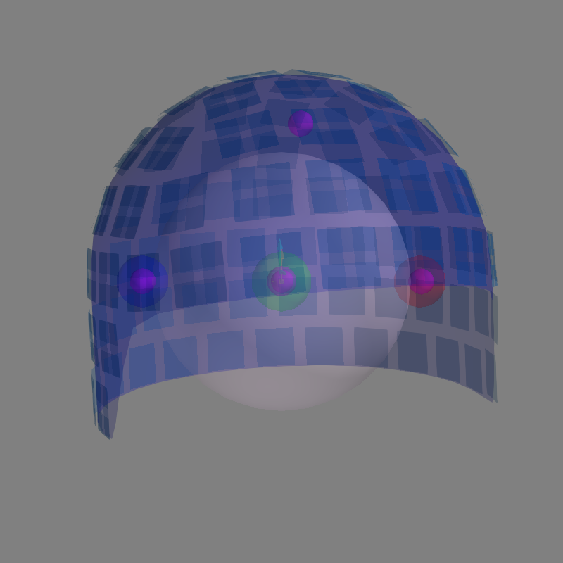
Let’s plot the positions and the orientations of the actual and the estimated dipoles

actual_amp = np.ones(len(dip))  # misc amp to create Dipole instance
actual_gof = np.ones(len(dip))  # misc GOF to create Dipole instance
dip_true = \
    mne.Dipole(dip.times, actual_pos, actual_amp, actual_ori, actual_gof)

fig = mne.viz.plot_alignment(evoked.info, bem=sphere, surfaces='inner_skull',
                             coord_frame='head', meg='helmet', show_axes=True)

# Plot the position and the orientation of the actual dipole
fig = mne.viz.plot_dipole_locations(dipoles=dip_true, mode='arrow',
                                    subject=subject, color=(0., 0., 0.),
                                    fig=fig)

# Plot the position and the orientation of the estimated dipole
fig = mne.viz.plot_dipole_locations(dipoles=dip, mode='arrow', subject=subject,
                                    color=(0.2, 1., 0.5), fig=fig)

mne.viz.set_3d_view(figure=fig, azimuth=70, elevation=80, distance=0.5)

Out:

    Triangle neighbors and vertex normals...
Getting helmet for system 306m

Total running time of the script: ( 0 minutes 31.481 seconds)

Estimated memory usage: 238 MB

Gallery generated by Sphinx-Gallery