mne_connectivity.viz.plot_sensors_connectivity#
- mne_connectivity.viz.plot_sensors_connectivity(info, con, picks=None, *, cbar_label='Connectivity', n_con=20, cmap='RdBu', min_distance=0.05)[source]#
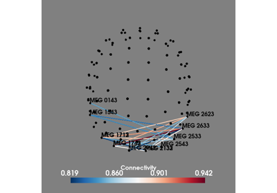
Visualize the sensor connectivity in 3D.
- Parameters:
- info
mne.Info The measurement info.
- con
array, shape (n_channels, n_channels) |Connectivity The connectivity data to plot.
- picks
str| array_like |slice|None Channels to include. Slices and lists of integers will be interpreted as channel indices. In lists, channel type strings (e.g.,
['meg',
'eeg']
) will pick channels of those types, channel name strings (e.g.,['MEG0111', 'MEG2623']will pick the given channels. Can also be the string values'all'to pick all channels, or'data'to pick data channels. None (default) will pick good data channels. Note that channels ininfo['bads']will be included if their names or indices are explicitly provided. Indices of selected channels.- cbar_label
str Label for the colorbar.
- n_con
int Number of strongest connections shown (default 20).
- cmap
str| instance ofmatplotlib.colors.Colormap Colormap for coloring connections by strength. If a str, must be a valid Matplotlib colormap (i.e. a valid key of
matplotlib.colormaps). Default is"RdBu".- min_distance
float The minimum distance required between two sensors to plot a connection between them, in meters. Default is 0.05 (i.e. 5 cm).
Added in version 0.8.
- info
- Returns:
- figinstance of Renderer
The 3D figure.
Examples using mne_connectivity.viz.plot_sensors_connectivity#
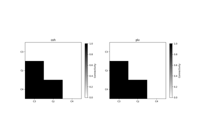
Comparing spectral connectivity computed over time or over trials