Artifact Correction Techniques

Here we artificially introduce several artifacts in a functional near-infrared spectroscopy (fNIRS) measurement and observe how artifact correction techniques attempt to correct the data.

# Authors: Robert Luke <mail@robertluke.net>
#
# License: BSD (3-clause)

import os

import matplotlib.pyplot as plt
import mne
import numpy as np
from mne.preprocessing.nirs import (
    optical_density,
    temporal_derivative_distribution_repair,
)

from mne_nirs.datasets import snirf_with_aux
from mne_nirs.io.snirf import read_snirf_aux_data
from mne_nirs.preprocessing import (
    detect_motion_artifacts,
    motion_correct_spline,
    motion_correct_wavelet,
)

Import data

Here we will work with the fNIRS motor data. We resample the data to make indexing exact times more convenient. We then convert the data to optical density to perform corrections on and plot these signals.

fnirs_data_folder = mne.datasets.fnirs_motor.data_path()
fnirs_cw_amplitude_dir = os.path.join(fnirs_data_folder, "Participant-1")
raw_intensity = mne.io.read_raw_nirx(fnirs_cw_amplitude_dir, verbose=True)
raw_intensity.load_data().resample(3, npad="auto")
raw_od = optical_density(raw_intensity)
new_annotations = mne.Annotations(
    [31, 187, 317], [8, 8, 8], ["Movement", "Movement", "Movement"]
)
raw_od.set_annotations(new_annotations)
raw_od.plot(n_channels=15, duration=400, show_scrollbars=False)

Loading /home/circleci/mne_data/MNE-fNIRS-motor-data/Participant-1

<MNEQtBrowser | RawNIRX, browsing 56 channels, 2974.7 s>

We can see some small artifacts in the above data from movement around 40, 190 and 240 seconds. However, this data is relatively clean so we will add some additional artifacts below.

Add artificial artifacts to data

Two common types of artifacts in NIRS data are spikes and baseline shifts. Spikes often occur when a person moves and the optode moves relative to the scalp and then returns to its original position. Baseline shifts occur if the optode moves relative to the scalp and does not return to its original position. We add a spike type artifact at 100 seconds and a baseline shift at 200 seconds to the data.

corrupted_data = raw_od.get_data()
corrupted_data[:, 298:302] = corrupted_data[:, 298:302] - 0.06
corrupted_data[:, 450:750] = corrupted_data[:, 450:750] + 0.03
corrupted_od = mne.io.RawArray(
    corrupted_data, raw_od.info, first_samp=raw_od.first_samp
)
new_annotations.append([95, 145, 245], [10, 10, 10], ["Spike", "Baseline", "Baseline"])
corrupted_od.set_annotations(new_annotations)

corrupted_od.plot(n_channels=15, duration=400, show_scrollbars=False)

<MNEQtBrowser | RawArray, browsing 56 channels, 2974.7 s>

Apply temporal derivative distribution repair

This approach corrects baseline shift and spike artifacts without the need for any user-supplied parameters [1].

corrected_tddr = temporal_derivative_distribution_repair(corrupted_od)
corrected_tddr.plot(n_channels=15, duration=400, show_scrollbars=False)

<MNEQtBrowser | RawArray, browsing 56 channels, 2974.7 s>

We can see in the data above that the introduced spikes and shifts are largely removed, but some residual smaller artifact remains. The same can be said for the artifacts in the original data.

Detect motion artifacts

The remaining techniques are ports of the Homer3 functions [2] and reproduce their output. They work in two stages: the motion artifacts are first detected and the flagged segments are then corrected. detect_motion_artifacts() flags a sample when, within a window of t_motion seconds, the signal changes by more than stdev_thresh times the standard deviation of its first derivative, or by more than amp_thresh optical density units. Each flagged sample is padded by t_mask seconds. Both wavelengths of a source-detector pair are evaluated together and share one mask. The default thresholds are those of Homer3, but suitable values depend on the sampling rate and noise level of the recording, so we use stricter values here that pick up the artifacts in this resampled data. The returned mask is True for clean samples and False for motion.

mask = detect_motion_artifacts(corrupted_od, stdev_thresh=10, amp_thresh=0.05)
print(f"{100 * (~mask).mean():.1f}% of samples flagged as motion artifacts")

0.4% of samples flagged as motion artifacts

Apply spline interpolation motion correction

Spline interpolation [3] fits a smoothing spline to each flagged segment, subtracts it, and shifts the segments so that the signal is continuous across their boundaries. It is most effective for baseline shifts. The smoothing parameter is the p of Homer3 and MATLAB’s csaps; the default of 0.99 is the value recommended in the literature. The correction is applied channel by channel using the mask computed above. If no mask is passed, the artifacts are detected with the default parameters.

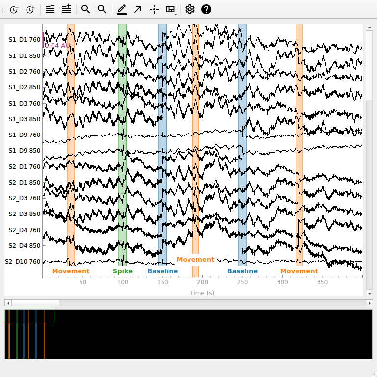
corrected_spline = motion_correct_spline(corrupted_od, mask=mask)
corrected_spline.plot(n_channels=15, duration=400, show_scrollbars=False)

<MNEQtBrowser | RawArray, browsing 56 channels, 2974.7 s>

The baseline shift is largely flattened and the spike is reduced. Because segments are shifted to match their neighbours, the absolute level of the optical density can differ from the original recording. This constant offset does not affect the haemoglobin changes computed later.

Apply wavelet motion correction

Wavelet correction [4] decomposes each channel with a translation-invariant wavelet transform and zeroes the coefficients that are outliers relative to the interquartile range, controlled by iqr. It targets spikes and leaves slow changes such as baseline shifts in place. This function requires the PyWavelets package.

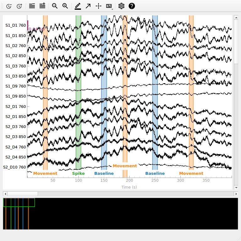
corrected_wavelet = motion_correct_wavelet(corrupted_od, iqr=1.5)
corrected_wavelet.plot(n_channels=15, duration=400, show_scrollbars=False)

<MNEQtBrowser | RawArray, browsing 56 channels, 2974.7 s>

The spike at 100 seconds is removed while the baseline shift remains, so the spline and wavelet methods are complementary [5] and are often applied one after the other.

Correct motion artifacts in real data

The artifacts above were added by hand. The recording from the auxiliary data example contains real ones, and the participant wore a head-mounted gyroscope that measured head rotation. Homer3’s default detection thresholds are conservative and flag almost nothing in this recording, so we lower stdev_thresh to 15. A more suitable value could be found by tuning it for the data at hand.

aux_file = snirf_with_aux.data_path()
raw_aux = mne.io.read_raw_snirf(aux_file).load_data()
od_aux = optical_density(raw_aux)
mask_aux = detect_motion_artifacts(od_aux, stdev_thresh=15)
corrected = {
    "Wavelet": motion_correct_wavelet(od_aux),
    "Spline": motion_correct_spline(od_aux, mask=mask_aux),
}
gyro = read_snirf_aux_data(aux_file, raw_aux)[[f"gyroscope_1_{a}" for a in "xyz"]]

pick = od_aux.ch_names.index("S8_D8 760")
times = od_aux.times / 60
fig, axes = plt.subplots(3, 1, sharex=True, figsize=(8, 7), layout="constrained")
for ax, (label, inst) in zip(axes, corrected.items()):
    ax.plot(times, od_aux.get_data(picks=pick)[0], lw=0.5, label="Original")
    ax.plot(times, inst.get_data(picks=pick)[0], lw=0.5, label=label)
    ax.set(ylabel="Optical density", title=f"{label} correction of S8_D8 760")
    ax.legend(loc="lower left")
axes[2].plot(times, np.linalg.norm(gyro, axis=1), color="k", lw=0.5)
axes[2].set(xlabel="Time (min)", ylabel="Head rotation", title="Gyroscope")
for ax in axes:
    ax.fill_between(
        times,
        0,
        1,
        where=~mask_aux[pick],
        color="r",
        alpha=0.3,
        transform=ax.get_xaxis_transform(),
    )

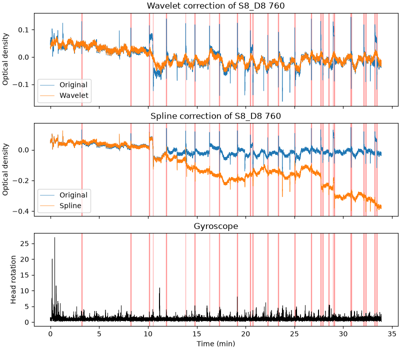
Some of the flagged periods (red) line up with bursts of head rotation, but not every movement disturbs this channel, and not every artifact comes with a large rotation. The wavelet correction removes the spikes while leaving slower changes in place. The spline correction, however, makes this channel worse: the corrected signal steps down after most artifacts, and the steps add up over the recording. Each artifact here is a spike followed by a dip that takes tens of seconds to recover, but only the spike is flagged, so each following segment is aligned to the bottom of the dip. Spline correction relies on the detection capturing each artifact in full [6][5], so check its output, for example by trying a longer t_mask, before relying on it.

References

[1]

Frank A Fishburn, Ruth S Ludlum, Chandan J Vaidya, and Andrei V Medvedev. Temporal derivative distribution repair (tddr): a motion correction method for fNIRS. NeuroImage, 184:171–179, 2019. doi:10.1016/j.neuroimage.2018.09.025.

[2]

Theodore J. Huppert, Solomon G. Diamond, Maria A. Franceschini, and David A. Boas. HomER: a review of time-series analysis methods for near-infrared spectroscopy of the brain. Applied Optics, 48(10):D280–D298, 2009. doi:10.1364/AO.48.00D280.

[3]

Felix Scholkmann, Sonja Spichtig, Thomas Muehlemann, and Martin Wolf. How to detect and reduce movement artifacts in near-infrared imaging using moving standard deviation and spline interpolation. Physiological Measurement, 31(5):649–662, 2010. doi:10.1088/0967-3334/31/5/004.

[4]

Behnam Molavi and Guy A. Dumont. Wavelet-based motion artifact removal for functional near-infrared spectroscopy. Physiological Measurement, 33(2):259–270, 2012. doi:10.1088/0967-3334/33/2/259.

[5] (1,2)

Sahar Jahani, Seyed K. Setarehdan, David A. Boas, and Meryem A. Yücel. Motion artifact detection and correction in functional near-infrared spectroscopy: a new hybrid method based on spline interpolation method and Savitzky-Golay filtering. Neurophotonics, 5(1):015003, 2018. doi:10.1117/1.NPh.5.1.015003.

[6]

Sabrina Brigadoi, Lisa Ceccherini, Simone Cutini, Fabio Scarpa, Pietro Scatturin, Juliette Selb, Louis Gagnon, David A. Boas, and Robert J. Cooper. Motion artifacts in functional near-infrared spectroscopy: a comparison of motion correction techniques applied to real cognitive data. NeuroImage, 85:181–191, 2014. doi:10.1016/j.neuroimage.2013.04.082.