Utilising Auxiliary Data

In this example we demonstrate how to load auxiliary data from a SNIRF file and include it in the design matrix for incorporating with your GLM analysis.

This example builds on the GLM tutorial. As such, we will not explain the GLM procedure in this example and refer readers to the detailed description above. Instead, we focus on extracting the auxiliary data and how this can be incorporated in to your analysis.

# sphinx_gallery_thumbnail_number = 2

# Authors: Robert Luke <code@robertluke.net>
#
# License: BSD (3-clause)

import matplotlib.pyplot as plt
import mne
import numpy as np
import pandas as pd
from nilearn.plotting import plot_design_matrix

from mne_nirs.channels import get_long_channels, get_short_channels
from mne_nirs.datasets.snirf_with_aux import data_path
from mne_nirs.experimental_design import make_first_level_design_matrix
from mne_nirs.io.snirf import read_snirf_aux_data

Import raw NIRS data

First we import the raw data. A different dataset is used from the previous GLM example that contains auxiliary data.

fnirs_snirf_file = data_path()
raw_intensity = mne.io.read_raw_snirf(fnirs_snirf_file).load_data()
raw_intensity.resample(0.7)

	General
	Filename(s)	2022-08-05_002.snirf
	MNE object type	RawSNIRF
	Measurement date	2022-08-05 at 13:10:58 UTC
	Participant	default
	Experimenter	Unknown
	Acquisition
	Duration	00:33:53 (HH:MM:SS)
	Sampling frequency	0.70 Hz
	Time points	1,424
	Channels
	fNIRS (CW amplitude)	56
	Head & sensor digitization	300 points
	Filters
	Highpass	0.00 Hz
	Lowpass	0.35 Hz

Clean up annotations before analysis

Next we update the annotations by assigning names to each trigger ID. Then we crop the recording to the section containing our experimental conditions.

raw_intensity.annotations.rename(
    {"1": "Control", "2": "Tapping_Left", "3": "Tapping_Right"}
)
raw_intensity.annotations.delete(raw_intensity.annotations.description == "15")
raw_intensity.annotations.set_durations(5)

<Annotations | 60 segments: Control (20), Tapping_Left (20), Tapping_Right ...>

Preprocess NIRS data

Next we convert the raw data to haemoglobin concentration.

raw_od = mne.preprocessing.nirs.optical_density(raw_intensity)
raw_haemo = mne.preprocessing.nirs.beer_lambert_law(raw_od, ppf=0.1)

We then split the data in to short channels which predominantly contain systemic responses and long channels which have both neural and systemic contributions.

short_chs = get_short_channels(raw_haemo)
raw_haemo = get_long_channels(raw_haemo)

Create design matrix

Relevant literature

For further discussion on design matrices see the Nilearn examples. Specifically the first level model example.

Next we create a model to fit our data to. The model consists of various components to model different things we assume contribute to the measured signal.

design_matrix = make_first_level_design_matrix(
    raw_haemo,
    drift_model="cosine",
    high_pass=0.005,  # Must be specified per experiment
    hrf_model="spm",
    stim_dur=5.0,
)

We also add the mean of the short channels to the design matrix. In theory these channels contain only systemic components, so including them in the design matrix allows us to estimate the neural component related to each experimental condition uncontaminated by systemic effects.

design_matrix["ShortHbO"] = np.mean(
    short_chs.copy().pick(picks="hbo").get_data(), axis=0
)

design_matrix["ShortHbR"] = np.mean(
    short_chs.copy().pick(picks="hbr").get_data(), axis=0
)

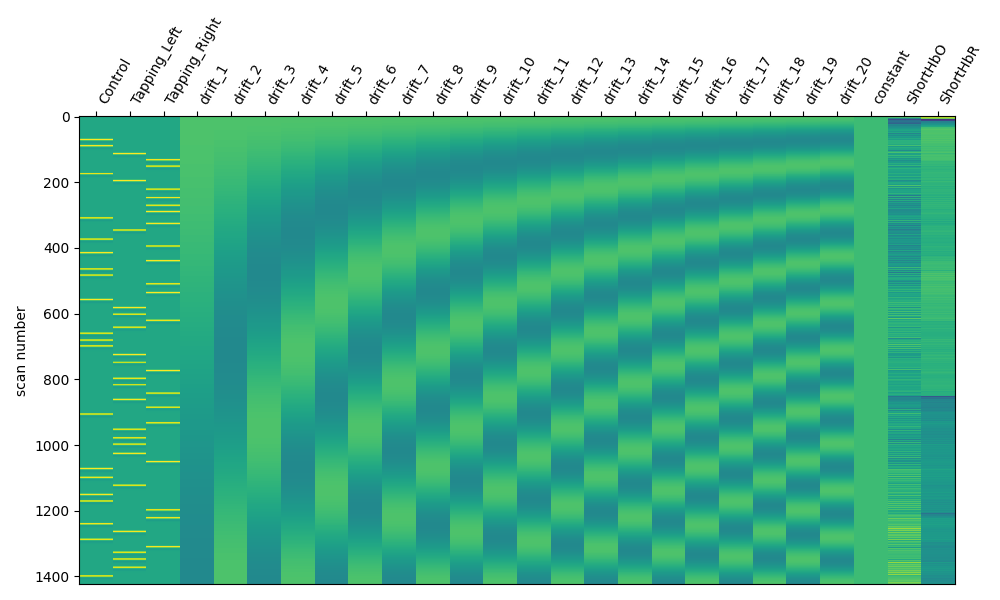
We can view the design matrix by printing the variable and we see that it includes the standard regressors, but does not yet contain any auxiliary data.

fig, ax1 = plt.subplots(figsize=(10, 6), nrows=1, ncols=1)
fig = plot_design_matrix(design_matrix, ax=ax1)

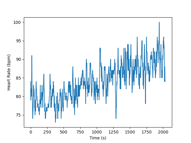
Load auxiliary data

The design matrix is a pandas data frame. As such, we wish to load the auxiliary data in the same format. The following function will load the SNIRF file and extract the auxiliary data. The auxiliary data can be sampled at a different rate to the raw fNIRS data, so this function will conveniently resample the data to the same rate as the raw fNIRS data.

aux_df = read_snirf_aux_data(fnirs_snirf_file, raw_haemo)

And you can verify the data looks reasonable by plotting individual fields.

plt.plot(raw_haemo.times, aux_df["HR"])
plt.xlabel("Time (s)")
plt.ylabel("Heart Rate (bpm)")

Text(38.347222222222214, 0.5, 'Heart Rate (bpm)')

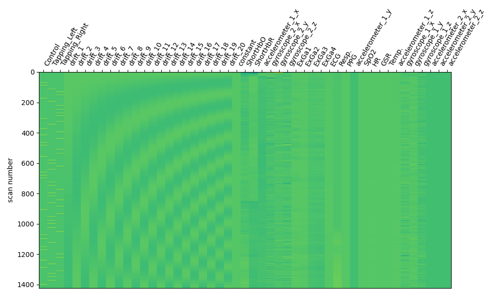
Include auxiliary data in design matrix

Finally we append the auxiliary data to the design matrix so that these can be included as regressors in a GLM analysis.

design_matrix = pd.concat([design_matrix, aux_df], axis=1)

And we can visually display the design matrix and verify the data is included.

fig, ax1 = plt.subplots(figsize=(10, 6), nrows=1, ncols=1)
fig = plot_design_matrix(design_matrix, ax=ax1)

Conclusion

We have demonstrated how to load auxiliary data from a SNIRF file. We illustrated how to include this data in your design matrix for further GLM analysis. We do not go through a full GLM analysis, instead the reader is directed to the dedicated GLM tutorial. The auxiliary data may need to be treated before being included in your analysis, for example you may need to normalise before inclusion in statistical analysis etc, but this is beyond the scope of this tutorial.

Estimated memory usage: 452 MB