Note
Click here to download the full example code
Visualising statistical significance thresholds on EEG data#
MNE-Python provides a range of tools for statistical hypothesis testing and the visualisation of the results. Here, we show a few options for exploratory and confirmatory tests - e.g., targeted t-tests, cluster-based permutation approaches (here with Threshold-Free Cluster Enhancement); and how to visualise the results.
The underlying data comes from [1]; we contrast long vs. short words. TFCE is described in [2].
import numpy as np
import matplotlib.pyplot as plt
from scipy.stats import ttest_ind

import mne
from mne.channels import find_ch_adjacency, make_1020_channel_selections
from mne.stats import spatio_temporal_cluster_test

np.random.seed(0)

# Load the data
path = mne.datasets.kiloword.data_path() / 'kword_metadata-epo.fif'
epochs = mne.read_epochs(path)
# These data are quite smooth, so to speed up processing we'll (unsafely!) just
# decimate them
epochs.decimate(4, verbose='error')
name = "NumberOfLetters"

# Split up the data by the median length in letters via the attached metadata
median_value = str(epochs.metadata[name].median())
long_words = epochs[name + " > " + median_value]
short_words = epochs[name + " < " + median_value]
Reading /home/circleci/mne_data/MNE-kiloword-data/kword_metadata-epo.fif ...
Isotrak not found
    Found the data of interest:
        t =    -100.00 ...     920.00 ms
        0 CTF compensation matrices available
Adding metadata with 8 columns
960 matching events found
No baseline correction applied
0 projection items activated
If we have a specific point in space and time we wish to test, it can be
convenient to convert the data into Pandas Dataframe format. In this case,
the mne.Epochs object has a convenient
mne.Epochs.to_data_frame() method, which returns a dataframe.
This dataframe can then be queried for specific time windows and sensors.
The extracted data can be submitted to standard statistical tests. Here,
we conduct t-tests on the difference between long and short words.
time_windows = ((.2, .25), (.35, .45))
elecs = ["Fz", "Cz", "Pz"]
index = ['condition', 'epoch', 'time']

# display the EEG data in Pandas format (first 5 rows)
print(epochs.to_data_frame(index=index)[elecs].head())

report = "{elec}, time: {tmin}-{tmax} s; t({df})={t_val:.3f}, p={p:.3f}"
print("\nTargeted statistical test results:")
for (tmin, tmax) in time_windows:
    long_df = long_words.copy().crop(tmin, tmax).to_data_frame(index=index)
    short_df = short_words.copy().crop(tmin, tmax).to_data_frame(index=index)
    for elec in elecs:
        # extract data
        A = long_df[elec].groupby("condition").mean()
        B = short_df[elec].groupby("condition").mean()

        # conduct t test
        t, p = ttest_ind(A, B)

        # display results
        format_dict = dict(elec=elec, tmin=tmin, tmax=tmax,
                           df=len(epochs.events) - 2, t_val=t, p=p)
        print(report.format(**format_dict))
channel                       Fz  ...        Pz
condition epoch time              ...
film      0     -0.096  0.453939  ...  0.222424
                -0.080  0.518939  ... -0.371515
                -0.064  0.811667  ...  0.250152
                -0.048  0.039697  ...  0.318030
                -0.032 -1.163030  ... -0.425152

[5 rows x 3 columns]

Targeted statistical test results:
Fz, time: 0.2-0.25 s; t(958)=-0.661, p=0.509
Cz, time: 0.2-0.25 s; t(958)=-2.682, p=0.007
Pz, time: 0.2-0.25 s; t(958)=-3.238, p=0.001
Fz, time: 0.35-0.45 s; t(958)=5.304, p=0.000
Cz, time: 0.35-0.45 s; t(958)=5.684, p=0.000
Pz, time: 0.35-0.45 s; t(958)=6.508, p=0.000
Absent specific hypotheses, we can also conduct an exploratory mass-univariate analysis at all sensors and time points. This requires correcting for multiple tests. MNE offers various methods for this; amongst them, cluster-based permutation methods allow deriving power from the spatio-temoral correlation structure of the data. Here, we use TFCE.
# Calculate adjacency matrix between sensors from their locations
adjacency, _ = find_ch_adjacency(epochs.info, "eeg")

# Extract data: transpose because the cluster test requires channels to be last
# In this case, inference is done over items. In the same manner, we could
# also conduct the test over, e.g., subjects.
X = [long_words.get_data().transpose(0, 2, 1),
     short_words.get_data().transpose(0, 2, 1)]
tfce = dict(start=.4, step=.4)  # ideally start and step would be smaller

# Calculate statistical thresholds
t_obs, clusters, cluster_pv, h0 = spatio_temporal_cluster_test(
    X, tfce, adjacency=adjacency,
    n_permutations=100)  # a more standard number would be 1000+
significant_points = cluster_pv.reshape(t_obs.shape).T < .05
print(str(significant_points.sum()) + " points selected by TFCE ...")
Could not find a adjacency matrix for the data. Computing adjacency based on Delaunay triangulations.
-- number of adjacent vertices : 29
stat_fun(H1): min=0.000001 max=80.917298
Running initial clustering …
Using 202 thresholds from 0.40 to 80.80 for TFCE computation (h_power=2.00, e_power=0.50)
Found 1856 clusters
0%| | Permuting : 0/99 [00:00<?, ?it/s]
1%|1 | Permuting : 1/99 [00:00<00:09, 9.89it/s]
2%|2 | Permuting : 2/99 [00:00<00:06, 15.02it/s]
3%|3 | Permuting : 3/99 [00:00<00:05, 18.15it/s]
4%|4 | Permuting : 4/99 [00:00<00:05, 17.11it/s]
5%|5 | Permuting : 5/99 [00:00<00:05, 16.56it/s]
6%|6 | Permuting : 6/99 [00:00<00:05, 16.20it/s]
7%|7 | Permuting : 7/99 [00:00<00:05, 17.43it/s]
8%|8 | Permuting : 8/99 [00:00<00:05, 16.99it/s]
9%|9 | Permuting : 9/99 [00:00<00:04, 18.02it/s]
10%|# | Permuting : 10/99 [00:00<00:04, 18.87it/s]
11%|#1 | Permuting : 11/99 [00:00<00:04, 18.30it/s]
12%|#2 | Permuting : 12/99 [00:00<00:04, 19.08it/s]
13%|#3 | Permuting : 13/99 [00:00<00:04, 18.54it/s]
14%|#4 | Permuting : 14/99 [00:00<00:04, 19.24it/s]
15%|#5 | Permuting : 15/99 [00:00<00:04, 17.69it/s]
16%|#6 | Permuting : 16/99 [00:00<00:04, 17.39it/s]
17%|#7 | Permuting : 17/99 [00:00<00:04, 18.03it/s]
18%|#8 | Permuting : 18/99 [00:00<00:04, 18.63it/s]
19%|#9 | Permuting : 19/99 [00:01<00:04, 18.26it/s]
20%|## | Permuting : 20/99 [00:01<00:04, 18.77it/s]
21%|##1 | Permuting : 21/99 [00:01<00:04, 17.58it/s]
22%|##2 | Permuting : 22/99 [00:01<00:04, 18.12it/s]
23%|##3 | Permuting : 23/99 [00:01<00:04, 17.83it/s]
24%|##4 | Permuting : 24/99 [00:01<00:04, 17.58it/s]
25%|##5 | Permuting : 25/99 [00:01<00:04, 18.09it/s]
26%|##6 | Permuting : 26/99 [00:01<00:03, 18.57it/s]
27%|##7 | Permuting : 27/99 [00:01<00:03, 18.26it/s]
28%|##8 | Permuting : 28/99 [00:01<00:03, 18.73it/s]
29%|##9 | Permuting : 29/99 [00:01<00:03, 18.42it/s]
30%|### | Permuting : 30/99 [00:01<00:03, 18.14it/s]
31%|###1 | Permuting : 31/99 [00:01<00:03, 18.59it/s]
32%|###2 | Permuting : 32/99 [00:01<00:03, 19.03it/s]
33%|###3 | Permuting : 33/99 [00:01<00:03, 18.71it/s]
34%|###4 | Permuting : 34/99 [00:01<00:03, 19.13it/s]
35%|###5 | Permuting : 35/99 [00:01<00:03, 18.81it/s]
36%|###6 | Permuting : 36/99 [00:01<00:03, 19.22it/s]
37%|###7 | Permuting : 37/99 [00:01<00:03, 18.89it/s]
38%|###8 | Permuting : 38/99 [00:02<00:03, 19.30it/s]
39%|###9 | Permuting : 39/99 [00:02<00:03, 18.97it/s]
40%|#### | Permuting : 40/99 [00:02<00:03, 18.67it/s]
41%|####1 | Permuting : 41/99 [00:02<00:03, 18.40it/s]
42%|####2 | Permuting : 42/99 [00:02<00:03, 18.80it/s]
43%|####3 | Permuting : 43/99 [00:02<00:03, 18.52it/s]
44%|####4 | Permuting : 44/99 [00:02<00:02, 18.91it/s]
45%|####5 | Permuting : 45/99 [00:02<00:02, 19.30it/s]
46%|####6 | Permuting : 46/99 [00:02<00:02, 19.68it/s]
47%|####7 | Permuting : 47/99 [00:02<00:02, 19.33it/s]
48%|####8 | Permuting : 48/99 [00:02<00:02, 18.38it/s]
49%|####9 | Permuting : 49/99 [00:02<00:02, 18.14it/s]
51%|##### | Permuting : 50/99 [00:02<00:02, 18.53it/s]
52%|#####1 | Permuting : 51/99 [00:02<00:02, 18.29it/s]
53%|#####2 | Permuting : 52/99 [00:02<00:02, 18.67it/s]
54%|#####3 | Permuting : 53/99 [00:02<00:02, 18.41it/s]
55%|#####4 | Permuting : 54/99 [00:02<00:02, 18.79it/s]
56%|#####5 | Permuting : 55/99 [00:02<00:02, 19.12it/s]
57%|#####6 | Permuting : 56/99 [00:03<00:02, 18.83it/s]
58%|#####7 | Permuting : 57/99 [00:03<00:02, 17.97it/s]
59%|#####8 | Permuting : 58/99 [00:03<00:02, 17.23it/s]
60%|#####9 | Permuting : 59/99 [00:03<00:02, 17.09it/s]
61%|###### | Permuting : 60/99 [00:03<00:02, 17.47it/s]
62%|######1 | Permuting : 61/99 [00:03<00:02, 17.85it/s]
63%|######2 | Permuting : 62/99 [00:03<00:02, 18.23it/s]
64%|######3 | Permuting : 63/99 [00:03<00:01, 18.02it/s]
65%|######4 | Permuting : 64/99 [00:03<00:01, 18.39it/s]
66%|######5 | Permuting : 65/99 [00:03<00:01, 18.76it/s]
67%|######6 | Permuting : 66/99 [00:03<00:01, 18.51it/s]
68%|######7 | Permuting : 67/99 [00:03<00:01, 18.27it/s]
69%|######8 | Permuting : 68/99 [00:03<00:01, 18.64it/s]
70%|######9 | Permuting : 69/99 [00:03<00:01, 18.40it/s]
71%|####### | Permuting : 70/99 [00:03<00:01, 17.62it/s]
72%|#######1 | Permuting : 71/99 [00:03<00:01, 17.45it/s]
73%|#######2 | Permuting : 72/99 [00:03<00:01, 17.30it/s]
74%|#######3 | Permuting : 73/99 [00:04<00:01, 17.15it/s]
75%|#######4 | Permuting : 74/99 [00:04<00:01, 17.01it/s]
76%|#######5 | Permuting : 75/99 [00:04<00:01, 16.87it/s]
77%|#######6 | Permuting : 76/99 [00:04<00:01, 16.29it/s]
78%|#######7 | Permuting : 77/99 [00:04<00:01, 16.67it/s]
79%|#######8 | Permuting : 78/99 [00:04<00:01, 16.11it/s]
80%|#######9 | Permuting : 79/99 [00:04<00:01, 16.47it/s]
81%|######## | Permuting : 80/99 [00:04<00:01, 15.93it/s]
82%|########1 | Permuting : 81/99 [00:04<00:01, 16.31it/s]
83%|########2 | Permuting : 82/99 [00:04<00:01, 16.23it/s]
84%|########3 | Permuting : 83/99 [00:04<00:00, 16.61it/s]
85%|########4 | Permuting : 84/99 [00:04<00:00, 16.50it/s]
86%|########5 | Permuting : 85/99 [00:04<00:00, 16.88it/s]
87%|########6 | Permuting : 86/99 [00:04<00:00, 16.76it/s]
88%|########7 | Permuting : 87/99 [00:04<00:00, 16.65it/s]
89%|########8 | Permuting : 88/99 [00:05<00:00, 16.55it/s]
90%|########9 | Permuting : 89/99 [00:05<00:00, 16.45it/s]
91%|######### | Permuting : 90/99 [00:05<00:00, 16.83it/s]
92%|#########1| Permuting : 91/99 [00:05<00:00, 17.20it/s]
93%|#########2| Permuting : 92/99 [00:05<00:00, 17.06it/s]
94%|#########3| Permuting : 93/99 [00:05<00:00, 16.46it/s]
95%|#########4| Permuting : 94/99 [00:05<00:00, 16.37it/s]
96%|#########5| Permuting : 95/99 [00:05<00:00, 16.75it/s]
97%|#########6| Permuting : 96/99 [00:05<00:00, 16.64it/s]
98%|#########7| Permuting : 97/99 [00:05<00:00, 17.01it/s]
99%|#########8| Permuting : 98/99 [00:05<00:00, 17.38it/s]
100%|##########| Permuting : 99/99 [00:05<00:00, 17.88it/s]
100%|##########| Permuting : 99/99 [00:05<00:00, 17.77it/s]
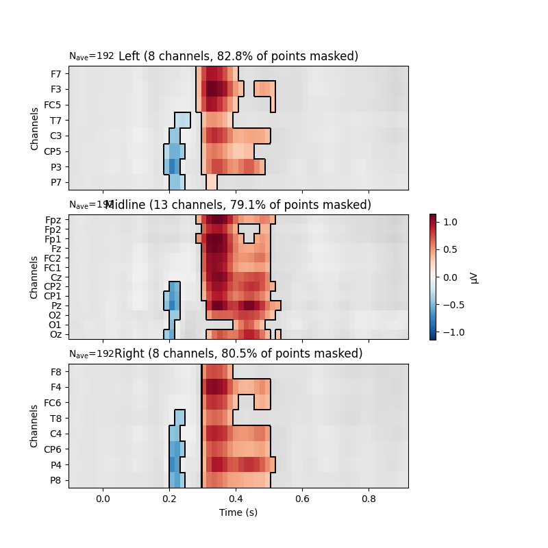
362 points selected by TFCE ...
The results of these mass univariate analyses can be visualised by plotting
mne.Evoked objects as images (via mne.Evoked.plot_image)
and masking points for significance.
Here, we group channels by Regions of Interest to facilitate localising
effects on the head.
# We need an evoked object to plot the image to be masked
evoked = mne.combine_evoked([long_words.average(), short_words.average()],
weights=[1, -1]) # calculate difference wave
time_unit = dict(time_unit="s")
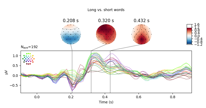
evoked.plot_joint(title="Long vs. short words", ts_args=time_unit,
topomap_args=time_unit) # show difference wave
# Create ROIs by checking channel labels
selections = make_1020_channel_selections(evoked.info, midline="12z")
# Visualize the results
fig, axes = plt.subplots(nrows=3, figsize=(8, 8))
axes = {sel: ax for sel, ax in zip(selections, axes.ravel())}
evoked.plot_image(axes=axes, group_by=selections, colorbar=False, show=False,
mask=significant_points, show_names="all", titles=None,
**time_unit)
plt.colorbar(axes["Left"].images[-1], ax=list(axes.values()), shrink=.3,
label="µV")
plt.show()
No projector specified for this dataset. Please consider the method self.add_proj.
References#
Total running time of the script: ( 0 minutes 11.531 seconds)
Estimated memory usage: 113 MB