Note
Click here to download the full example code
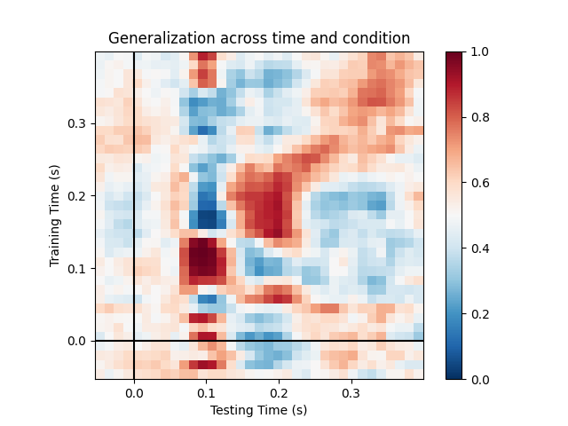
Decoding sensor space data with generalization across time and conditions#
This example runs the analysis described in [1]. It illustrates how one can fit a linear classifier to identify a discriminatory topography at a given time instant and subsequently assess whether this linear model can accurately predict all of the time samples of a second set of conditions.
# Authors: Jean-Remi King <jeanremi.king@gmail.com>
#          Alexandre Gramfort <alexandre.gramfort@inria.fr>
#          Denis Engemann <denis.engemann@gmail.com>
#
# License: BSD-3-Clause
import matplotlib.pyplot as plt

from sklearn.pipeline import make_pipeline
from sklearn.preprocessing import StandardScaler
from sklearn.linear_model import LogisticRegression

import mne
from mne.datasets import sample
from mne.decoding import GeneralizingEstimator

print(__doc__)

# Preprocess data
data_path = sample.data_path()
# Load and filter data, set up epochs
meg_path = data_path / 'MEG' / 'sample'
raw_fname = meg_path / 'sample_audvis_filt-0-40_raw.fif'
events_fname = meg_path / 'sample_audvis_filt-0-40_raw-eve.fif'
raw = mne.io.read_raw_fif(raw_fname, preload=True)
picks = mne.pick_types(raw.info, meg=True, exclude='bads')  # Pick MEG channels
raw.filter(1., 30., fir_design='firwin')  # Band pass filtering signals
events = mne.read_events(events_fname)
event_id = {'Auditory/Left': 1, 'Auditory/Right': 2,
            'Visual/Left': 3, 'Visual/Right': 4}
tmin = -0.050
tmax = 0.400
# decimate to make the example faster to run, but then use verbose='error' in
# the Epochs constructor to suppress warning about decimation causing aliasing
decim = 2
epochs = mne.Epochs(raw, events, event_id=event_id, tmin=tmin, tmax=tmax,
                    proj=True, picks=picks, baseline=None, preload=True,
                    reject=dict(mag=5e-12), decim=decim, verbose='error')
Opening raw data file /home/circleci/mne_data/MNE-sample-data/MEG/sample/sample_audvis_filt-0-40_raw.fif...
    Read a total of 4 projection items:
        PCA-v1 (1 x 10²)  idle
        PCA-v2 (1 x 10²)  idle
        PCA-v3 (1 x 10²)  idle
        Average EEG reference (1 x 60)  idle
    Range : 6450 ... 48149 =     42.956 ...   320.665 secs
Ready.
Reading 0 ... 41699  =      0.000 ...   277.709 secs...
Filtering raw data in 1 contiguous segment
Setting up band-pass filter from 1 - 30 Hz

FIR filter parameters
---------------------
Designing a one-pass, zero-phase, non-causal bandpass filter:
- Windowed time-domain design (firwin) method
- Hamming window with 0.0194 passband ripple and 53 dB stopband attenuation
- Lower passband edge: 1.00
- Lower transition bandwidth: 1.00 Hz (-6 dB cutoff frequency: 0.50 Hz)
- Upper passband edge: 30.00 Hz
- Upper transition bandwidth: 7.50 Hz (-6 dB cutoff frequency: 33.75 Hz)
- Filter length: 497 samples (3.310 sec)

[Parallel(n_jobs=1)]: Using backend SequentialBackend with 1 concurrent workers.
[Parallel(n_jobs=1)]: Done   1 out of   1 | elapsed:    0.0s remaining:    0.0s
[Parallel(n_jobs=1)]: Done   2 out of   2 | elapsed:    0.0s remaining:    0.0s
[Parallel(n_jobs=1)]: Done   3 out of   3 | elapsed:    0.0s remaining:    0.0s
[Parallel(n_jobs=1)]: Done   4 out of   4 | elapsed:    0.0s remaining:    0.0s
[Parallel(n_jobs=1)]: Done 366 out of 366 | elapsed:    0.6s finished
We will train the classifier on all left visual vs auditory trials and test on all right visual vs auditory trials.
clf = make_pipeline(
    StandardScaler(),
    LogisticRegression(solver='liblinear')  # liblinear is faster than lbfgs
)
time_gen = GeneralizingEstimator(clf, scoring='roc_auc', n_jobs=None,
                                 verbose=True)

# Fit classifiers on the epochs where the stimulus was presented to the left.
# Note that the experimental condition y indicates auditory or visual
time_gen.fit(X=epochs['Left'].get_data(),
             y=epochs['Left'].events[:, 2] > 2)
  0%|          | Fitting GeneralizingEstimator : 0/35 [00:00<?,       ?it/s]
  6%|5         | Fitting GeneralizingEstimator : 2/35 [00:00<00:00,   58.43it/s]
 14%|#4        | Fitting GeneralizingEstimator : 5/35 [00:00<00:00,   73.99it/s]
 20%|##        | Fitting GeneralizingEstimator : 7/35 [00:00<00:00,   68.89it/s]
 31%|###1      | Fitting GeneralizingEstimator : 11/35 [00:00<00:00,   82.31it/s]
 43%|####2     | Fitting GeneralizingEstimator : 15/35 [00:00<00:00,   90.27it/s]
 51%|#####1    | Fitting GeneralizingEstimator : 18/35 [00:00<00:00,   90.02it/s]
 60%|######    | Fitting GeneralizingEstimator : 21/35 [00:00<00:00,   89.85it/s]
 71%|#######1  | Fitting GeneralizingEstimator : 25/35 [00:00<00:00,   94.00it/s]
 77%|#######7  | Fitting GeneralizingEstimator : 27/35 [00:00<00:00,   89.31it/s]
 89%|########8 | Fitting GeneralizingEstimator : 31/35 [00:00<00:00,   92.95it/s]
 97%|#########7| Fitting GeneralizingEstimator : 34/35 [00:00<00:00,   92.52it/s]
100%|##########| Fitting GeneralizingEstimator : 35/35 [00:00<00:00,   91.98it/s]
Score on the epochs where the stimulus was presented to the right.
scores = time_gen.score(X=epochs['Right'].get_data(),
                        y=epochs['Right'].events[:, 2] > 2)
  0%|          | Scoring GeneralizingEstimator : 0/1225 [00:00<?,       ?it/s]
  1%|1         | Scoring GeneralizingEstimator : 18/1225 [00:00<00:02,  527.49it/s]
  3%|3         | Scoring GeneralizingEstimator : 40/1225 [00:00<00:02,  590.55it/s]
  5%|5         | Scoring GeneralizingEstimator : 62/1225 [00:00<00:01,  610.09it/s]
  7%|6         | Scoring GeneralizingEstimator : 85/1225 [00:00<00:01,  629.49it/s]
  9%|8         | Scoring GeneralizingEstimator : 107/1225 [00:00<00:01,  634.47it/s]
 11%|#         | Scoring GeneralizingEstimator : 130/1225 [00:00<00:01,  643.49it/s]
 12%|#2        | Scoring GeneralizingEstimator : 153/1225 [00:00<00:01,  650.00it/s]
 14%|#4        | Scoring GeneralizingEstimator : 176/1225 [00:00<00:01,  654.74it/s]
 16%|#6        | Scoring GeneralizingEstimator : 198/1225 [00:00<00:01,  654.23it/s]
 18%|#8        | Scoring GeneralizingEstimator : 221/1225 [00:00<00:01,  657.86it/s]
 20%|#9        | Scoring GeneralizingEstimator : 244/1225 [00:00<00:01,  660.82it/s]
 22%|##1       | Scoring GeneralizingEstimator : 267/1225 [00:00<00:01,  663.12it/s]
 24%|##3       | Scoring GeneralizingEstimator : 291/1225 [00:00<00:01,  668.01it/s]
 26%|##5       | Scoring GeneralizingEstimator : 314/1225 [00:00<00:01,  669.46it/s]
 28%|##7       | Scoring GeneralizingEstimator : 337/1225 [00:00<00:01,  670.66it/s]
 29%|##9       | Scoring GeneralizingEstimator : 360/1225 [00:00<00:01,  671.64it/s]
 31%|###1      | Scoring GeneralizingEstimator : 383/1225 [00:00<00:01,  672.63it/s]
 33%|###3      | Scoring GeneralizingEstimator : 405/1225 [00:00<00:01,  671.05it/s]
 35%|###5      | Scoring GeneralizingEstimator : 429/1225 [00:00<00:01,  674.43it/s]
 37%|###6      | Scoring GeneralizingEstimator : 452/1225 [00:00<00:01,  674.77it/s]
 39%|###8      | Scoring GeneralizingEstimator : 475/1225 [00:00<00:01,  675.29it/s]
 41%|####      | Scoring GeneralizingEstimator : 498/1225 [00:00<00:01,  675.61it/s]
 43%|####2     | Scoring GeneralizingEstimator : 521/1225 [00:00<00:01,  675.83it/s]
 44%|####4     | Scoring GeneralizingEstimator : 544/1225 [00:00<00:01,  676.14it/s]
 46%|####6     | Scoring GeneralizingEstimator : 568/1225 [00:00<00:00,  678.52it/s]
 48%|####8     | Scoring GeneralizingEstimator : 591/1225 [00:00<00:00,  678.77it/s]
 50%|#####     | Scoring GeneralizingEstimator : 614/1225 [00:00<00:00,  679.03it/s]
 52%|#####2    | Scoring GeneralizingEstimator : 637/1225 [00:00<00:00,  679.18it/s]
 54%|#####3    | Scoring GeneralizingEstimator : 660/1225 [00:00<00:00,  679.30it/s]
 56%|#####5    | Scoring GeneralizingEstimator : 682/1225 [00:01<00:00,  677.35it/s]
 58%|#####7    | Scoring GeneralizingEstimator : 705/1225 [00:01<00:00,  677.56it/s]
 59%|#####9    | Scoring GeneralizingEstimator : 728/1225 [00:01<00:00,  677.84it/s]
 61%|######1   | Scoring GeneralizingEstimator : 751/1225 [00:01<00:00,  677.99it/s]
 63%|######3   | Scoring GeneralizingEstimator : 774/1225 [00:01<00:00,  678.25it/s]
 65%|######5   | Scoring GeneralizingEstimator : 797/1225 [00:01<00:00,  678.47it/s]
 67%|######6   | Scoring GeneralizingEstimator : 820/1225 [00:01<00:00,  678.54it/s]
 69%|######8   | Scoring GeneralizingEstimator : 843/1225 [00:01<00:00,  678.76it/s]
 71%|#######   | Scoring GeneralizingEstimator : 866/1225 [00:01<00:00,  678.87it/s]
 73%|#######2  | Scoring GeneralizingEstimator : 889/1225 [00:01<00:00,  678.88it/s]
 74%|#######4  | Scoring GeneralizingEstimator : 912/1225 [00:01<00:00,  678.87it/s]
 76%|#######6  | Scoring GeneralizingEstimator : 935/1225 [00:01<00:00,  678.96it/s]
 78%|#######8  | Scoring GeneralizingEstimator : 957/1225 [00:01<00:00,  677.35it/s]
 80%|########  | Scoring GeneralizingEstimator : 981/1225 [00:01<00:00,  679.23it/s]
 82%|########1 | Scoring GeneralizingEstimator : 1003/1225 [00:01<00:00,  677.68it/s]
 84%|########3 | Scoring GeneralizingEstimator : 1026/1225 [00:01<00:00,  677.75it/s]
 86%|########5 | Scoring GeneralizingEstimator : 1049/1225 [00:01<00:00,  677.70it/s]
 88%|########7 | Scoring GeneralizingEstimator : 1072/1225 [00:01<00:00,  676.37it/s]
 89%|########9 | Scoring GeneralizingEstimator : 1095/1225 [00:01<00:00,  676.35it/s]
 91%|#########1| Scoring GeneralizingEstimator : 1118/1225 [00:01<00:00,  676.32it/s]
 93%|#########3| Scoring GeneralizingEstimator : 1141/1225 [00:01<00:00,  676.46it/s]
 95%|#########5| Scoring GeneralizingEstimator : 1164/1225 [00:01<00:00,  676.57it/s]
 97%|#########6| Scoring GeneralizingEstimator : 1187/1225 [00:01<00:00,  676.56it/s]
 99%|#########8| Scoring GeneralizingEstimator : 1210/1225 [00:01<00:00,  676.53it/s]
100%|##########| Scoring GeneralizingEstimator : 1225/1225 [00:01<00:00,  676.57it/s]
100%|##########| Scoring GeneralizingEstimator : 1225/1225 [00:01<00:00,  674.74it/s]
Plot
fig, ax = plt.subplots(1)
im = ax.matshow(scores, vmin=0, vmax=1., cmap='RdBu_r', origin='lower',
                extent=epochs.times[[0, -1, 0, -1]])
ax.axhline(0., color='k')
ax.axvline(0., color='k')
ax.xaxis.set_ticks_position('bottom')
ax.set_xlabel('Testing Time (s)')
ax.set_ylabel('Training Time (s)')
ax.set_title('Generalization across time and condition')
plt.colorbar(im, ax=ax)
plt.show()
References#
Total running time of the script: ( 0 minutes 6.620 seconds)
Estimated memory usage: 129 MB