Note
Go to the end to download the full example code
Compute and visualize ERDS maps#
This example calculates and displays ERDS maps of event-related EEG data. ERDS (sometimes also written as ERD/ERS) is short for event-related desynchronization (ERD) and event-related synchronization (ERS) [1]. Conceptually, ERD corresponds to a decrease in power in a specific frequency band relative to a baseline. Similarly, ERS corresponds to an increase in power. An ERDS map is a time/frequency representation of ERD/ERS over a range of frequencies [2]. ERDS maps are also known as ERSP (event-related spectral perturbation) [3].
In this example, we use an EEG BCI data set containing two different motor imagery tasks (imagined hand and feet movement). Our goal is to generate ERDS maps for each of the two tasks.
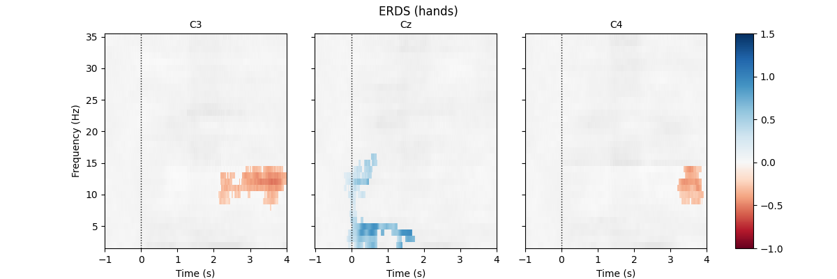
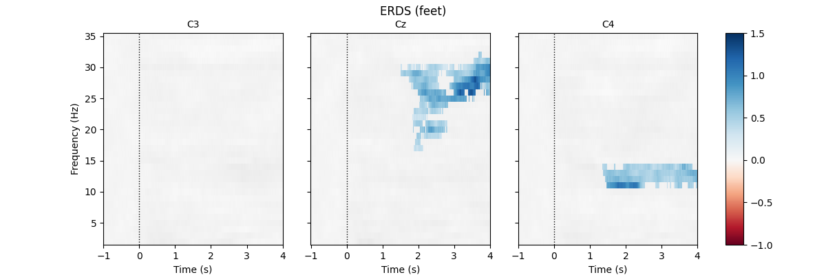
First, we load the data and create epochs of 5s length. The data set contains multiple channels, but we will only consider C3, Cz, and C4. We compute maps containing frequencies ranging from 2 to 35Hz. We map ERD to red color and ERS to blue color, which is customary in many ERDS publications. Finally, we perform cluster-based permutation tests to estimate significant ERDS values (corrected for multiple comparisons within channels).
# Authors: Clemens Brunner <clemens.brunner@gmail.com>
#          Felix Klotzsche <klotzsche@cbs.mpg.de>
#
# License: BSD-3-Clause
As usual, we import everything we need.
import numpy as np
import matplotlib.pyplot as plt
from matplotlib.colors import TwoSlopeNorm
import pandas as pd
import seaborn as sns
import mne
from mne.datasets import eegbci
from mne.io import concatenate_raws, read_raw_edf
from mne.time_frequency import tfr_multitaper
from mne.stats import permutation_cluster_1samp_test as pcluster_test
First, we load and preprocess the data. We use runs 6, 10, and 14 from subject 1 (these runs contains hand and feet motor imagery).
fnames = eegbci.load_data(subject=1, runs=(6, 10, 14))
raw = concatenate_raws([read_raw_edf(f, preload=True) for f in fnames])

raw.rename_channels(lambda x: x.strip('.'))  # remove dots from channel names

events, _ = mne.events_from_annotations(raw, event_id=dict(T1=2, T2=3))
Exception ignored in: <_io.FileIO name='/home/circleci/project/mne/data/eegbci_checksums.txt' mode='rb' closefd=True>
Traceback (most recent call last):
  File "<decorator-gen-568>", line 12, in load_data
ResourceWarning: unclosed file <_io.BufferedReader name='/home/circleci/project/mne/data/eegbci_checksums.txt'>
Extracting EDF parameters from /home/circleci/mne_data/MNE-eegbci-data/files/eegmmidb/1.0.0/S001/S001R06.edf...
EDF file detected
Setting channel info structure...
Creating raw.info structure...
Reading 0 ... 19999  =      0.000 ...   124.994 secs...
Extracting EDF parameters from /home/circleci/mne_data/MNE-eegbci-data/files/eegmmidb/1.0.0/S001/S001R10.edf...
EDF file detected
Setting channel info structure...
Creating raw.info structure...
Reading 0 ... 19999  =      0.000 ...   124.994 secs...
Extracting EDF parameters from /home/circleci/mne_data/MNE-eegbci-data/files/eegmmidb/1.0.0/S001/S001R14.edf...
EDF file detected
Setting channel info structure...
Creating raw.info structure...
Reading 0 ... 19999  =      0.000 ...   124.994 secs...
Used Annotations descriptions: ['T1', 'T2']
Now we can create 5-second epochs around events of interest.
Not setting metadata
45 matching events found
No baseline correction applied
0 projection items activated
Using data from preloaded Raw for 45 events and 961 original time points ...
0 bad epochs dropped
Here we set suitable values for computing ERDS maps. Note especially the
cnorm variable, which sets up an asymmetric colormap where the middle
color is mapped to zero, even though zero is not the middle value of the
colormap range. This does two things: it ensures that zero values will be
plotted in white (given that below we select the RdBu colormap), and it
makes synchronization and desynchronization look equally prominent in the
plots, even though their extreme values are of different magnitudes.
freqs = np.arange(2, 36)  # frequencies from 2-35Hz
vmin, vmax = -1, 1.5  # set min and max ERDS values in plot
baseline = (-1, 0)  # baseline interval (in s)
cnorm = TwoSlopeNorm(vmin=vmin, vcenter=0, vmax=vmax)  # min, center & max ERDS

kwargs = dict(n_permutations=100, step_down_p=0.05, seed=1,
              buffer_size=None, out_type='mask')  # for cluster test
Finally, we perform time/frequency decomposition over all epochs.
tfr = tfr_multitaper(epochs, freqs=freqs, n_cycles=freqs, use_fft=True,
                     return_itc=False, average=False, decim=2)
tfr.crop(tmin, tmax).apply_baseline(baseline, mode="percent")

for event in event_ids:
    # select desired epochs for visualization
    tfr_ev = tfr[event]
    fig, axes = plt.subplots(1, 4, figsize=(12, 4),
                             gridspec_kw={"width_ratios": [10, 10, 10, 1]})
    for ch, ax in enumerate(axes[:-1]):  # for each channel
        # positive clusters
        _, c1, p1, _ = pcluster_test(tfr_ev.data[:, ch], tail=1, **kwargs)
        # negative clusters
        _, c2, p2, _ = pcluster_test(tfr_ev.data[:, ch], tail=-1, **kwargs)

        # note that we keep clusters with p <= 0.05 from the combined clusters
        # of two independent tests; in this example, we do not correct for
        # these two comparisons
        c = np.stack(c1 + c2, axis=2)  # combined clusters
        p = np.concatenate((p1, p2))  # combined p-values
        mask = c[..., p <= 0.05].any(axis=-1)

        # plot TFR (ERDS map with masking)
        tfr_ev.average().plot([ch], cmap="RdBu", cnorm=cnorm, axes=ax,
                              colorbar=False, show=False, mask=mask,
                              mask_style="mask")

        ax.set_title(epochs.ch_names[ch], fontsize=10)
        ax.axvline(0, linewidth=1, color="black", linestyle=":")  # event
        if ch != 0:
            ax.set_ylabel("")
            ax.set_yticklabels("")
    fig.colorbar(axes[0].images[-1], cax=axes[-1]).ax.set_yscale("linear")
    fig.suptitle(f"ERDS ({event})")
    plt.show()
[Parallel(n_jobs=1)]: Using backend SequentialBackend with 1 concurrent workers.
[Parallel(n_jobs=1)]: Done   1 out of   1 | elapsed:    0.2s remaining:    0.0s
[Parallel(n_jobs=1)]: Done   2 out of   2 | elapsed:    0.5s remaining:    0.0s
[Parallel(n_jobs=1)]: Done   3 out of   3 | elapsed:    0.7s remaining:    0.0s
[Parallel(n_jobs=1)]: Done   3 out of   3 | elapsed:    0.7s finished
Not setting metadata
Applying baseline correction (mode: percent)
Using a threshold of 1.724718
stat_fun(H1): min=-8.523637 max=3.197747
Running initial clustering …
Found 78 clusters

  0%|          | Permuting : 0/99 [00:00<?,       ?it/s]
  6%|6         | Permuting : 6/99 [00:00<00:00,  172.07it/s]
 13%|#3        | Permuting : 13/99 [00:00<00:00,  189.90it/s]
 19%|#9        | Permuting : 19/99 [00:00<00:00,  185.46it/s]
 27%|##7       | Permuting : 27/99 [00:00<00:00,  199.22it/s]
 37%|###7      | Permuting : 37/99 [00:00<00:00,  220.45it/s]
 48%|####8     | Permuting : 48/99 [00:00<00:00,  240.25it/s]
 61%|######    | Permuting : 60/99 [00:00<00:00,  259.25it/s]
 72%|#######1  | Permuting : 71/99 [00:00<00:00,  268.98it/s]
 83%|########2 | Permuting : 82/99 [00:00<00:00,  276.64it/s]
 95%|#########4| Permuting : 94/99 [00:00<00:00,  286.34it/s]
100%|##########| Permuting : 99/99 [00:00<00:00,  278.91it/s]
Step-down-in-jumps iteration #1 found 0 clusters to exclude from subsequent iterations
Using a threshold of -1.724718
stat_fun(H1): min=-8.523637 max=3.197747
Running initial clustering …
Found 65 clusters

  0%|          | Permuting : 0/99 [00:00<?,       ?it/s]
 11%|#1        | Permuting : 11/99 [00:00<00:00,  325.15it/s]
 22%|##2       | Permuting : 22/99 [00:00<00:00,  324.85it/s]
 34%|###4      | Permuting : 34/99 [00:00<00:00,  335.52it/s]
 44%|####4     | Permuting : 44/99 [00:00<00:00,  324.87it/s]
 56%|#####5    | Permuting : 55/99 [00:00<00:00,  325.09it/s]
 66%|######5   | Permuting : 65/99 [00:00<00:00,  319.56it/s]
 74%|#######3  | Permuting : 73/99 [00:00<00:00,  305.86it/s]
 82%|########1 | Permuting : 81/99 [00:00<00:00,  295.64it/s]
 90%|########9 | Permuting : 89/99 [00:00<00:00,  287.64it/s]
 97%|#########6| Permuting : 96/99 [00:00<00:00,  277.63it/s]
100%|##########| Permuting : 99/99 [00:00<00:00,  284.10it/s]
Step-down-in-jumps iteration #1 found 1 cluster to exclude from subsequent iterations

  0%|          | Permuting : 0/99 [00:00<?,       ?it/s]
 11%|#1        | Permuting : 11/99 [00:00<00:00,  324.46it/s]
 22%|##2       | Permuting : 22/99 [00:00<00:00,  325.09it/s]
 33%|###3      | Permuting : 33/99 [00:00<00:00,  325.38it/s]
 44%|####4     | Permuting : 44/99 [00:00<00:00,  325.28it/s]
 55%|#####4    | Permuting : 54/99 [00:00<00:00,  318.83it/s]
 66%|######5   | Permuting : 65/99 [00:00<00:00,  320.04it/s]
 78%|#######7  | Permuting : 77/99 [00:00<00:00,  325.94it/s]
 88%|########7 | Permuting : 87/99 [00:00<00:00,  321.54it/s]
 97%|#########6| Permuting : 96/99 [00:00<00:00,  313.73it/s]
100%|##########| Permuting : 99/99 [00:00<00:00,  313.78it/s]
Step-down-in-jumps iteration #2 found 0 additional clusters to exclude from subsequent iterations
No baseline correction applied
Using a threshold of 1.724718
stat_fun(H1): min=-4.573067 max=3.687727
Running initial clustering …
Found 85 clusters

  0%|          | Permuting : 0/99 [00:00<?,       ?it/s]
  8%|8         | Permuting : 8/99 [00:00<00:00,  235.77it/s]
 16%|#6        | Permuting : 16/99 [00:00<00:00,  235.26it/s]
 25%|##5       | Permuting : 25/99 [00:00<00:00,  246.16it/s]
 33%|###3      | Permuting : 33/99 [00:00<00:00,  243.69it/s]
 41%|####1     | Permuting : 41/99 [00:00<00:00,  242.06it/s]
 51%|#####     | Permuting : 50/99 [00:00<00:00,  246.38it/s]
 59%|#####8    | Permuting : 58/99 [00:00<00:00,  244.78it/s]
 69%|######8   | Permuting : 68/99 [00:00<00:00,  252.16it/s]
 81%|########  | Permuting : 80/99 [00:00<00:00,  266.03it/s]
 91%|######### | Permuting : 90/99 [00:00<00:00,  269.76it/s]
100%|##########| Permuting : 99/99 [00:00<00:00,  277.12it/s]
100%|##########| Permuting : 99/99 [00:00<00:00,  271.31it/s]
Step-down-in-jumps iteration #1 found 1 cluster to exclude from subsequent iterations

  0%|          | Permuting : 0/99 [00:00<?,       ?it/s]
  9%|9         | Permuting : 9/99 [00:00<00:00,  265.24it/s]
 20%|##        | Permuting : 20/99 [00:00<00:00,  296.26it/s]
 31%|###1      | Permuting : 31/99 [00:00<00:00,  306.44it/s]
 41%|####1     | Permuting : 41/99 [00:00<00:00,  303.72it/s]
 53%|#####2    | Permuting : 52/99 [00:00<00:00,  308.61it/s]
 65%|######4   | Permuting : 64/99 [00:00<00:00,  317.50it/s]
 77%|#######6  | Permuting : 76/99 [00:00<00:00,  323.81it/s]
 88%|########7 | Permuting : 87/99 [00:00<00:00,  324.09it/s]
100%|##########| Permuting : 99/99 [00:00<00:00,  330.86it/s]
100%|##########| Permuting : 99/99 [00:00<00:00,  327.25it/s]
Step-down-in-jumps iteration #2 found 0 additional clusters to exclude from subsequent iterations
Using a threshold of -1.724718
stat_fun(H1): min=-4.573067 max=3.687727
Running initial clustering …
Found 57 clusters

  0%|          | Permuting : 0/99 [00:00<?,       ?it/s]
 11%|#1        | Permuting : 11/99 [00:00<00:00,  324.36it/s]
 23%|##3       | Permuting : 23/99 [00:00<00:00,  339.75it/s]
 31%|###1      | Permuting : 31/99 [00:00<00:00,  303.86it/s]
 39%|###9      | Permuting : 39/99 [00:00<00:00,  285.65it/s]
 47%|####7     | Permuting : 47/99 [00:00<00:00,  274.81it/s]
 56%|#####5    | Permuting : 55/99 [00:00<00:00,  267.61it/s]
 64%|######3   | Permuting : 63/99 [00:00<00:00,  262.49it/s]
 72%|#######1  | Permuting : 71/99 [00:00<00:00,  258.68it/s]
 80%|#######9  | Permuting : 79/99 [00:00<00:00,  255.77it/s]
 90%|########9 | Permuting : 89/99 [00:00<00:00,  260.80it/s]
100%|##########| Permuting : 99/99 [00:00<00:00,  267.62it/s]
100%|##########| Permuting : 99/99 [00:00<00:00,  268.10it/s]
Step-down-in-jumps iteration #1 found 0 clusters to exclude from subsequent iterations
No baseline correction applied
Using a threshold of 1.724718
stat_fun(H1): min=-6.599131 max=3.329547
Running initial clustering …
Found 64 clusters

  0%|          | Permuting : 0/99 [00:00<?,       ?it/s]
  9%|9         | Permuting : 9/99 [00:00<00:00,  265.11it/s]
 19%|#9        | Permuting : 19/99 [00:00<00:00,  280.69it/s]
 29%|##9       | Permuting : 29/99 [00:00<00:00,  286.17it/s]
 39%|###9      | Permuting : 39/99 [00:00<00:00,  288.95it/s]
 49%|####9     | Permuting : 49/99 [00:00<00:00,  290.62it/s]
 60%|#####9    | Permuting : 59/99 [00:00<00:00,  291.64it/s]
 70%|######9   | Permuting : 69/99 [00:00<00:00,  292.42it/s]
 78%|#######7  | Permuting : 77/99 [00:00<00:00,  284.19it/s]
 89%|########8 | Permuting : 88/99 [00:00<00:00,  289.82it/s]
100%|##########| Permuting : 99/99 [00:00<00:00,  294.39it/s]
100%|##########| Permuting : 99/99 [00:00<00:00,  292.81it/s]
Step-down-in-jumps iteration #1 found 0 clusters to exclude from subsequent iterations
Using a threshold of -1.724718
stat_fun(H1): min=-6.599131 max=3.329547
Running initial clustering …
Found 64 clusters

  0%|          | Permuting : 0/99 [00:00<?,       ?it/s]
 10%|#         | Permuting : 10/99 [00:00<00:00,  295.12it/s]
 20%|##        | Permuting : 20/99 [00:00<00:00,  295.64it/s]
 30%|###       | Permuting : 30/99 [00:00<00:00,  295.43it/s]
 41%|####1     | Permuting : 41/99 [00:00<00:00,  303.24it/s]
 53%|#####2    | Permuting : 52/99 [00:00<00:00,  307.90it/s]
 63%|######2   | Permuting : 62/99 [00:00<00:00,  305.44it/s]
 73%|#######2  | Permuting : 72/99 [00:00<00:00,  303.64it/s]
 84%|########3 | Permuting : 83/99 [00:00<00:00,  306.68it/s]
 95%|#########4| Permuting : 94/99 [00:00<00:00,  309.05it/s]
100%|##########| Permuting : 99/99 [00:00<00:00,  309.98it/s]
Step-down-in-jumps iteration #1 found 0 clusters to exclude from subsequent iterations
No baseline correction applied
Using a threshold of 1.713872
stat_fun(H1): min=-3.687815 max=3.369164
Running initial clustering …
Found 66 clusters

  0%|          | Permuting : 0/99 [00:00<?,       ?it/s]
 10%|#         | Permuting : 10/99 [00:00<00:00,  295.18it/s]
 20%|##        | Permuting : 20/99 [00:00<00:00,  295.49it/s]
 30%|###       | Permuting : 30/99 [00:00<00:00,  295.93it/s]
 40%|####      | Permuting : 40/99 [00:00<00:00,  295.98it/s]
 51%|#####     | Permuting : 50/99 [00:00<00:00,  296.02it/s]
 62%|######1   | Permuting : 61/99 [00:00<00:00,  301.37it/s]
 71%|#######   | Permuting : 70/99 [00:00<00:00,  295.43it/s]
 81%|########  | Permuting : 80/99 [00:00<00:00,  295.56it/s]
 91%|######### | Permuting : 90/99 [00:00<00:00,  295.66it/s]
100%|##########| Permuting : 99/99 [00:00<00:00,  298.39it/s]
100%|##########| Permuting : 99/99 [00:00<00:00,  297.64it/s]
Step-down-in-jumps iteration #1 found 0 clusters to exclude from subsequent iterations
Using a threshold of -1.713872
stat_fun(H1): min=-3.687815 max=3.369164
Running initial clustering …
Found 75 clusters

  0%|          | Permuting : 0/99 [00:00<?,       ?it/s]
 10%|#         | Permuting : 10/99 [00:00<00:00,  295.67it/s]
 20%|##        | Permuting : 20/99 [00:00<00:00,  293.56it/s]
 31%|###1      | Permuting : 31/99 [00:00<00:00,  303.89it/s]
 41%|####1     | Permuting : 41/99 [00:00<00:00,  301.86it/s]
 53%|#####2    | Permuting : 52/99 [00:00<00:00,  307.07it/s]
 63%|######2   | Permuting : 62/99 [00:00<00:00,  305.03it/s]
 74%|#######3  | Permuting : 73/99 [00:00<00:00,  308.35it/s]
 85%|########4 | Permuting : 84/99 [00:00<00:00,  310.70it/s]
 95%|#########4| Permuting : 94/99 [00:00<00:00,  308.74it/s]
100%|##########| Permuting : 99/99 [00:00<00:00,  308.55it/s]
100%|##########| Permuting : 99/99 [00:00<00:00,  307.68it/s]
Step-down-in-jumps iteration #1 found 0 clusters to exclude from subsequent iterations
No baseline correction applied
Using a threshold of 1.713872
stat_fun(H1): min=-5.046259 max=5.406477
Running initial clustering …
Found 98 clusters

  0%|          | Permuting : 0/99 [00:00<?,       ?it/s]
  9%|9         | Permuting : 9/99 [00:00<00:00,  265.23it/s]
 19%|#9        | Permuting : 19/99 [00:00<00:00,  280.97it/s]
 30%|###       | Permuting : 30/99 [00:00<00:00,  296.51it/s]
 40%|####      | Permuting : 40/99 [00:00<00:00,  296.21it/s]
 52%|#####1    | Permuting : 51/99 [00:00<00:00,  302.58it/s]
 63%|######2   | Permuting : 62/99 [00:00<00:00,  306.83it/s]
 73%|#######2  | Permuting : 72/99 [00:00<00:00,  305.04it/s]
 84%|########3 | Permuting : 83/99 [00:00<00:00,  308.11it/s]
 94%|#########3| Permuting : 93/99 [00:00<00:00,  306.46it/s]
100%|##########| Permuting : 99/99 [00:00<00:00,  306.94it/s]
100%|##########| Permuting : 99/99 [00:00<00:00,  305.52it/s]
Step-down-in-jumps iteration #1 found 1 cluster to exclude from subsequent iterations

  0%|          | Permuting : 0/99 [00:00<?,       ?it/s]
  9%|9         | Permuting : 9/99 [00:00<00:00,  265.85it/s]
 20%|##        | Permuting : 20/99 [00:00<00:00,  296.47it/s]
 30%|###       | Permuting : 30/99 [00:00<00:00,  296.47it/s]
 41%|####1     | Permuting : 41/99 [00:00<00:00,  304.22it/s]
 52%|#####1    | Permuting : 51/99 [00:00<00:00,  302.39it/s]
 64%|######3   | Permuting : 63/99 [00:00<00:00,  312.36it/s]
 75%|#######4  | Permuting : 74/99 [00:00<00:00,  314.58it/s]
 85%|########4 | Permuting : 84/99 [00:00<00:00,  311.88it/s]
 96%|#########5| Permuting : 95/99 [00:00<00:00,  313.61it/s]
100%|##########| Permuting : 99/99 [00:00<00:00,  314.96it/s]
Step-down-in-jumps iteration #2 found 0 additional clusters to exclude from subsequent iterations
Using a threshold of -1.713872
stat_fun(H1): min=-5.046259 max=5.406477
Running initial clustering …
Found 66 clusters

  0%|          | Permuting : 0/99 [00:00<?,       ?it/s]
  9%|9         | Permuting : 9/99 [00:00<00:00,  266.03it/s]
 18%|#8        | Permuting : 18/99 [00:00<00:00,  266.15it/s]
 26%|##6       | Permuting : 26/99 [00:00<00:00,  255.58it/s]
 34%|###4      | Permuting : 34/99 [00:00<00:00,  250.04it/s]
 43%|####3     | Permuting : 43/99 [00:00<00:00,  253.60it/s]
 53%|#####2    | Permuting : 52/99 [00:00<00:00,  255.89it/s]
 60%|#####9    | Permuting : 59/99 [00:00<00:00,  247.88it/s]
 70%|######9   | Permuting : 69/99 [00:00<00:00,  255.04it/s]
 80%|#######9  | Permuting : 79/99 [00:00<00:00,  260.62it/s]
 91%|######### | Permuting : 90/99 [00:00<00:00,  268.64it/s]
100%|##########| Permuting : 99/99 [00:00<00:00,  272.42it/s]
100%|##########| Permuting : 99/99 [00:00<00:00,  268.88it/s]
Step-down-in-jumps iteration #1 found 0 clusters to exclude from subsequent iterations
No baseline correction applied
Using a threshold of 1.713872
stat_fun(H1): min=-5.964817 max=4.078953
Running initial clustering …
Found 92 clusters

  0%|          | Permuting : 0/99 [00:00<?,       ?it/s]
  8%|8         | Permuting : 8/99 [00:00<00:00,  236.51it/s]
 16%|#6        | Permuting : 16/99 [00:00<00:00,  236.39it/s]
 24%|##4       | Permuting : 24/99 [00:00<00:00,  236.45it/s]
 34%|###4      | Permuting : 34/99 [00:00<00:00,  252.45it/s]
 45%|####5     | Permuting : 45/99 [00:00<00:00,  268.48it/s]
 56%|#####5    | Permuting : 55/99 [00:00<00:00,  273.42it/s]
 63%|######2   | Permuting : 62/99 [00:00<00:00,  262.42it/s]
 73%|#######2  | Permuting : 72/99 [00:00<00:00,  267.44it/s]
 84%|########3 | Permuting : 83/99 [00:00<00:00,  275.05it/s]
 94%|#########3| Permuting : 93/99 [00:00<00:00,  277.61it/s]
100%|##########| Permuting : 99/99 [00:00<00:00,  274.08it/s]
100%|##########| Permuting : 99/99 [00:00<00:00,  271.85it/s]
Step-down-in-jumps iteration #1 found 1 cluster to exclude from subsequent iterations

  0%|          | Permuting : 0/99 [00:00<?,       ?it/s]
 10%|#         | Permuting : 10/99 [00:00<00:00,  294.62it/s]
 21%|##1       | Permuting : 21/99 [00:00<00:00,  310.45it/s]
 32%|###2      | Permuting : 32/99 [00:00<00:00,  315.61it/s]
 43%|####3     | Permuting : 43/99 [00:00<00:00,  318.35it/s]
 56%|#####5    | Permuting : 55/99 [00:00<00:00,  326.15it/s]
 67%|######6   | Permuting : 66/99 [00:00<00:00,  325.85it/s]
 77%|#######6  | Permuting : 76/99 [00:00<00:00,  320.84it/s]
 89%|########8 | Permuting : 88/99 [00:00<00:00,  326.00it/s]
100%|##########| Permuting : 99/99 [00:00<00:00,  326.30it/s]
100%|##########| Permuting : 99/99 [00:00<00:00,  324.97it/s]
Step-down-in-jumps iteration #2 found 0 additional clusters to exclude from subsequent iterations
Using a threshold of -1.713872
stat_fun(H1): min=-5.964817 max=4.078953
Running initial clustering …
Found 52 clusters

  0%|          | Permuting : 0/99 [00:00<?,       ?it/s]
 10%|#         | Permuting : 10/99 [00:00<00:00,  294.91it/s]
 22%|##2       | Permuting : 22/99 [00:00<00:00,  325.74it/s]
 33%|###3      | Permuting : 33/99 [00:00<00:00,  325.82it/s]
 44%|####4     | Permuting : 44/99 [00:00<00:00,  325.79it/s]
 55%|#####4    | Permuting : 54/99 [00:00<00:00,  319.22it/s]
 64%|######3   | Permuting : 63/99 [00:00<00:00,  309.19it/s]
 73%|#######2  | Permuting : 72/99 [00:00<00:00,  302.15it/s]
 84%|########3 | Permuting : 83/99 [00:00<00:00,  305.70it/s]
 94%|#########3| Permuting : 93/99 [00:00<00:00,  304.38it/s]
100%|##########| Permuting : 99/99 [00:00<00:00,  304.21it/s]
100%|##########| Permuting : 99/99 [00:00<00:00,  305.17it/s]
Step-down-in-jumps iteration #1 found 0 clusters to exclude from subsequent iterations
No baseline correction applied
Similar to Epochs objects, we can also export data from
EpochsTFR and AverageTFR objects
to a Pandas DataFrame. By default, the time
column of the exported data frame is in milliseconds. Here, to be consistent
with the time-frequency plots, we want to keep it in seconds, which we can
achieve by setting time_format=None:
df = tfr.to_data_frame(time_format=None)
df.head()
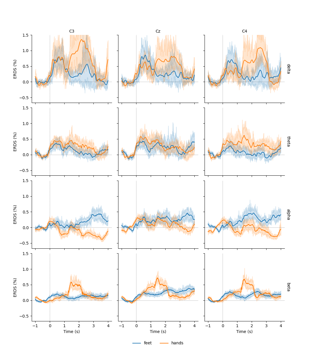
This allows us to use additional plotting functions like
seaborn.lineplot() to plot confidence bands:
df = tfr.to_data_frame(time_format=None, long_format=True)

# Map to frequency bands:
freq_bounds = {'_': 0,
               'delta': 3,
               'theta': 7,
               'alpha': 13,
               'beta': 35,
               'gamma': 140}
df['band'] = pd.cut(df['freq'], list(freq_bounds.values()),
                    labels=list(freq_bounds)[1:])

# Filter to retain only relevant frequency bands:
freq_bands_of_interest = ['delta', 'theta', 'alpha', 'beta']
df = df[df.band.isin(freq_bands_of_interest)]
df['band'] = df['band'].cat.remove_unused_categories()

# Order channels for plotting:
df['channel'] = df['channel'].cat.reorder_categories(('C3', 'Cz', 'C4'),
                                                     ordered=True)

g = sns.FacetGrid(df, row='band', col='channel', margin_titles=True)
g.map(sns.lineplot, 'time', 'value', 'condition', n_boot=10)
axline_kw = dict(color='black', linestyle='dashed', linewidth=0.5, alpha=0.5)
g.map(plt.axhline, y=0, **axline_kw)
g.map(plt.axvline, x=0, **axline_kw)
g.set(ylim=(None, 1.5))
g.set_axis_labels("Time (s)", "ERDS (%)")
g.set_titles(col_template="{col_name}", row_template="{row_name}")
g.add_legend(ncol=2, loc='lower center')
g.fig.subplots_adjust(left=0.1, right=0.9, top=0.9, bottom=0.08)
Converting "condition" to "category"...
Converting "epoch" to "category"...
Converting "channel" to "category"...
Converting "ch_type" to "category"...
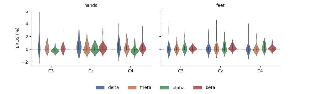
Having the data as a DataFrame also facilitates subsetting, grouping, and other transforms. Here, we use seaborn to plot the average ERDS in the motor imagery interval as a function of frequency band and imagery condition:
df_mean = (df.query('time > 1')
             .groupby(['condition', 'epoch', 'band', 'channel'])[['value']]
             .mean()
             .reset_index())

g = sns.FacetGrid(df_mean, col='condition', col_order=['hands', 'feet'],
                  margin_titles=True)
g = (g.map(sns.violinplot, 'channel', 'value', 'band', n_boot=10,
           palette='deep', order=['C3', 'Cz', 'C4'],
           hue_order=freq_bands_of_interest,
           linewidth=0.5).add_legend(ncol=4, loc='lower center'))

g.map(plt.axhline, **axline_kw)
g.set_axis_labels("", "ERDS (%)")
g.set_titles(col_template="{col_name}", row_template="{row_name}")
g.fig.subplots_adjust(left=0.1, right=0.9, top=0.9, bottom=0.3)
References#
Total running time of the script: ( 0 minutes 33.468 seconds)
Estimated memory usage: 229 MB