Note
Go to the end to download the full example code.
Using the event system to link figures#
Many of MNE-Python’s figures are interactive. For example, you can select channels or scroll through time. The event system allows you to link figures together so that interacting with one figure will simultaneously update another figure.
In this example, we’ll be looking at linking a topomap plot with a source estimate plot, such that selecting the time in one will also update the time in the other, as well as hooking our own custom plot into MNE-Python’s event system.
Since the figures on our website don’t have any interaction capabilities, this example will only work properly when run in an interactive environment.
# Author: Marijn van Vliet <w.m.vanvliet@gmail.com>
#
# License: BSD-3-Clause
# Copyright the MNE-Python contributors.
import matplotlib.pyplot as plt

import mne
from mne.viz.ui_events import TimeChange, link, publish, subscribe

# Turn on interactivity
plt.ion()
Linking interactive plots#
We load sensor-level and source-level data for the MNE-Sample dataset and create two plots that have sliders controlling the time-point that is shown. By default, both figures are independent, but we will link the event channels of the figures together, so that moving the slider in one figure will also move the slider in the other.
data_path = mne.datasets.sample.data_path()
evokeds_fname = data_path / "MEG" / "sample" / "sample_audvis-ave.fif"
evokeds = mne.read_evokeds(evokeds_fname)
for ev in evokeds:
ev.apply_baseline()
avg_evokeds = mne.combine_evoked(evokeds, "nave")
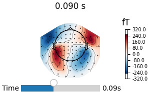
fig1 = avg_evokeds.plot_topomap("interactive")
stc_fname = data_path / "MEG" / "sample" / "sample_audvis-meg-eeg"
stc = mne.read_source_estimate(stc_fname)
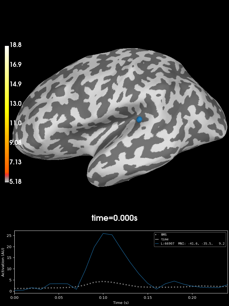
fig2 = stc.plot("sample", subjects_dir=data_path / "subjects")
link(fig1, fig2) # link the event channels
Reading /home/circleci/mne_data/MNE-sample-data/MEG/sample/sample_audvis-ave.fif ...
    Read a total of 4 projection items:
        PCA-v1 (1 x 10²) active
        PCA-v2 (1 x 10²) active
        PCA-v3 (1 x 10²) active
        Average EEG reference (1 x 60) active
    Found the data of interest:
        t =    -199.80 ...     499.49 ms (Left Auditory)
        0 CTF compensation matrices available
        nave = 55 - aspect type = 100
Projections have already been applied. Setting proj attribute to True.
No baseline correction applied
    Read a total of 4 projection items:
        PCA-v1 (1 x 10²) active
        PCA-v2 (1 x 10²) active
        PCA-v3 (1 x 10²) active
        Average EEG reference (1 x 60) active
    Found the data of interest:
        t =    -199.80 ...     499.49 ms (Right Auditory)
        0 CTF compensation matrices available
        nave = 61 - aspect type = 100
Projections have already been applied. Setting proj attribute to True.
No baseline correction applied
    Read a total of 4 projection items:
        PCA-v1 (1 x 10²) active
        PCA-v2 (1 x 10²) active
        PCA-v3 (1 x 10²) active
        Average EEG reference (1 x 60) active
    Found the data of interest:
        t =    -199.80 ...     499.49 ms (Left visual)
        0 CTF compensation matrices available
        nave = 67 - aspect type = 100
Projections have already been applied. Setting proj attribute to True.
No baseline correction applied
    Read a total of 4 projection items:
        PCA-v1 (1 x 10²) active
        PCA-v2 (1 x 10²) active
        PCA-v3 (1 x 10²) active
        Average EEG reference (1 x 60) active
    Found the data of interest:
        t =    -199.80 ...     499.49 ms (Right visual)
        0 CTF compensation matrices available
        nave = 58 - aspect type = 100
Projections have already been applied. Setting proj attribute to True.
No baseline correction applied
Applying baseline correction (mode: mean)
Applying baseline correction (mode: mean)
Applying baseline correction (mode: mean)
Applying baseline correction (mode: mean)
Using control points [ 5.17909658  6.18448887 18.83197989]
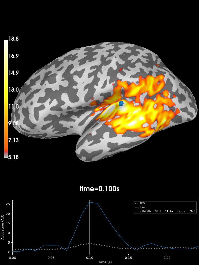
Overlaying one figure over another#
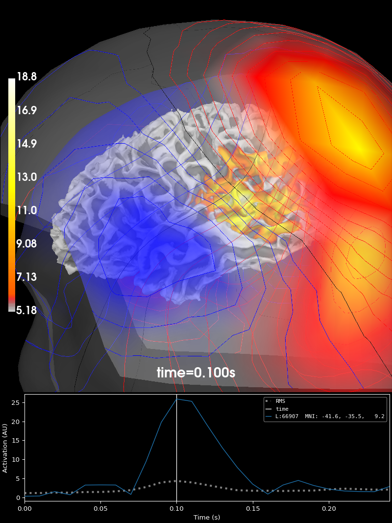
A common scenario in which the UI event system comes in handy is when plotting multiple things in the same figure. For example, if we want to draw the magnetic fieldlines on top of a source estimate, we can link the UI event channels together, so that when a different time is selected, both the source estimate and the fieldlines are updated together.
fig_brain = stc.plot("sample", subjects_dir=data_path / "subjects", surface="white")
fig_brain.show_view(distance=400)  # zoom out a little

field_map = mne.make_field_map(
    avg_evokeds,
    trans=data_path / "MEG" / "sample" / "sample_audvis_raw-trans.fif",
    subject="sample",
    subjects_dir=data_path / "subjects",
)
fig_field = mne.viz.plot_evoked_field(
    avg_evokeds,
    field_map,
    alpha=0.2,
    fig=fig_brain,  # plot inside the existing source estimate figure
    time_label=None,  # there is already a time label in the figure
)

link(fig_brain, fig_field)
fig_brain.set_time(0.1)  # updates both source estimate and field lines
Using control points [ 5.17909658  6.18448887 18.83197989]
Using surface from /home/circleci/mne_data/MNE-sample-data/subjects/sample/bem/sample-5120-5120-5120-bem.fif.
Getting helmet for system 306m
Prepare EEG mapping...
Computing dot products for 59 electrodes...
Computing dot products for 2562 surface locations...
Field mapping data ready
    Preparing the mapping matrix...
    Truncating at 21/59 components to omit less than 0.001 (0.00097)
    The map has an average electrode reference (2562 channels)
Prepare MEG mapping...
Computing dot products for 305 coils...
Computing dot products for 304 surface locations...
Field mapping data ready
    Preparing the mapping matrix...
    Truncating at 210/305 components to omit less than 0.0001 (9.9e-05)
Hooking a custom plot into the event system#
In MNE-Python, each figure has an associated event channel. Drawing routines can
publish events on the channel and receive events
by subscribe-ing to the channel. When
subscribing to an event on a channel, you specify a callback function to be called
whenever a drawing routine publishes that event on the event channel.
The events are modeled after matplotlib’s event system. Each event has a string name (the snake-case version of its class name) and a list of relevant values. For example, the “time_change” event should have the new time as a value. Values can be any python object. When publishing an event, the publisher creates a new instance of the event’s class. When subscribing to an event, having to dig up and import the correct class is a bit of a hassle. Following matplotlib’s example, subscribers use the string name of the event to refer to it.
Below, we create a custom plot and then make it publish and subscribe to
TimeChange events so it can work together with the
plots we created earlier.
# Recreate the earlier plots
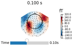
fig3 = avg_evokeds.plot_topomap("interactive")
fig4 = stc.plot("sample", subjects_dir=data_path / "subjects")
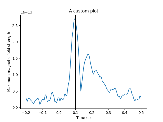
# Create a custom plot
fig5, ax = plt.subplots()
ax.plot(avg_evokeds.times, avg_evokeds.pick("mag").data.max(axis=0))
time_bar = ax.axvline(0, color="black") # Our time slider
ax.set_xlabel("Time (s)")
ax.set_ylabel("Maximum magnetic field strength")
ax.set_title("A custom plot")
def on_motion_notify(mpl_event):
"""Respond to matplotlib's mouse event.
Publishes an MNE-Python TimeChange event. When the mouse goes out of bounds, the
xdata will be None, which is a special case that needs to be handled.
"""
if mpl_event.xdata is not None:
publish(fig5, TimeChange(time=mpl_event.xdata))
def on_time_change(event):
"""Respond to MNE-Python's TimeChange event. Updates the plot."""
time_bar.set_xdata([event.time])
fig5.canvas.draw() # update the figure
# Setup the events for the curstom plot. Moving the mouse will trigger a
# matplotlib event, which we will respond to by publishing an MNE-Python UI
# event. Upon receiving a UI event, we will move the vertical line.
plt.connect("motion_notify_event", on_motion_notify)
subscribe(fig5, "time_change", on_time_change)
# Link all the figures together.
link(fig3, fig4, fig5)
# Method calls like this also emit the appropriate UI event.
fig4.set_time(0.1)
Using control points [ 5.17909658 6.18448887 18.83197989]
Total running time of the script: (0 minutes 19.391 seconds)
Estimated memory usage: 27 MB