Note
Go to the end to download the full example code.
Compute Power Spectral Density of inverse solution from single epochs#
Compute PSD of dSPM inverse solution on single trial epochs restricted to a brain label. The PSD is computed using a multi-taper method with Discrete Prolate Spheroidal Sequence (DPSS) windows.
# Author: Martin Luessi <mluessi@nmr.mgh.harvard.edu>
#
# License: BSD-3-Clause
# Copyright the MNE-Python contributors.
import matplotlib.pyplot as plt

import mne
from mne.datasets import sample
from mne.minimum_norm import compute_source_psd_epochs, read_inverse_operator

print(__doc__)

data_path = sample.data_path()
meg_path = data_path / "MEG" / "sample"
fname_inv = meg_path / "sample_audvis-meg-oct-6-meg-inv.fif"
fname_raw = meg_path / "sample_audvis_raw.fif"
fname_event = meg_path / "sample_audvis_raw-eve.fif"
label_name = "Aud-lh"
fname_label = meg_path / "labels" / f"{label_name}.label"
subjects_dir = data_path / "subjects"

event_id, tmin, tmax = 1, -0.2, 0.5
snr = 1.0  # use smaller SNR for raw data
lambda2 = 1.0 / snr**2
method = "dSPM"  # use dSPM method (could also be MNE or sLORETA)

# Load data
inverse_operator = read_inverse_operator(fname_inv)
label = mne.read_label(fname_label)
raw = mne.io.read_raw_fif(fname_raw)
events = mne.read_events(fname_event)

# Set up pick list
include = []
raw.info["bads"] += ["EEG 053"]  # bads + 1 more

# pick MEG channels
picks = mne.pick_types(
    raw.info, meg=True, eeg=False, stim=False, eog=True, include=include, exclude="bads"
)
# Read epochs
epochs = mne.Epochs(
    raw,
    events,
    event_id,
    tmin,
    tmax,
    picks=picks,
    baseline=(None, 0),
    reject=dict(mag=4e-12, grad=4000e-13, eog=150e-6),
)

# define frequencies of interest
fmin, fmax = 0.0, 70.0
bandwidth = 4.0  # bandwidth of the windows in Hz
Reading inverse operator decomposition from /home/circleci/mne_data/MNE-sample-data/MEG/sample/sample_audvis-meg-oct-6-meg-inv.fif...
    Reading inverse operator info...
    [done]
    Reading inverse operator decomposition...
    [done]
    305 x 305 full covariance (kind = 1) found.
    Read a total of 4 projection items:
        PCA-v1 (1 x 10²) active
        PCA-v2 (1 x 10²) active
        PCA-v3 (1 x 10²) active
        Average EEG reference (1 x 60) active
    Noise covariance matrix read.
    22494 x 22494 diagonal covariance (kind = 2) found.
    Source covariance matrix read.
    22494 x 22494 diagonal covariance (kind = 6) found.
    Orientation priors read.
    22494 x 22494 diagonal covariance (kind = 5) found.
    Depth priors read.
    Did not find the desired covariance matrix (kind = 3)
    Reading a source space...
    Computing patch statistics...
    Patch information added...
    Distance information added...
    [done]
    Reading a source space...
    Computing patch statistics...
    Patch information added...
    Distance information added...
    [done]
    2 source spaces read
    Read a total of 4 projection items:
        PCA-v1 (1 x 10²) active
        PCA-v2 (1 x 10²) active
        PCA-v3 (1 x 10²) active
        Average EEG reference (1 x 60) active
    Source spaces transformed to the inverse solution coordinate frame
Opening raw data file /home/circleci/mne_data/MNE-sample-data/MEG/sample/sample_audvis_raw.fif...
    Read a total of 3 projection items:
        PCA-v1 (1 x 10²)  idle
        PCA-v2 (1 x 10²)  idle
        PCA-v3 (1 x 10²)  idle
    Range : 25800 ... 192599 =     42.956 ...   320.670 secs
Ready.
Not setting metadata
72 matching events found
Setting baseline interval to [-0.19979521315838786, 0.0] s
Applying baseline correction (mode: mean)
Created an SSP operator (subspace dimension = 3)
3 projection items activated
Compute source space PSD in label#
- ..note:: By using “return_generator=True” stcs will be a generator object
instead of a list. This allows us so to iterate without having to keep everything in memory.
n_epochs_use = 10
stcs = compute_source_psd_epochs(
    epochs[:n_epochs_use],
    inverse_operator,
    lambda2=lambda2,
    method=method,
    fmin=fmin,
    fmax=fmax,
    bandwidth=bandwidth,
    label=label,
    return_generator=True,
    verbose=True,
)

# compute average PSD over the first 10 epochs
psd_avg = 0.0
for i, stc in enumerate(stcs):
    psd_avg += stc.data
psd_avg /= n_epochs_use
freqs = stc.times  # the frequencies are stored here
stc.data = psd_avg  # overwrite the last epoch's data with the average
Considering frequencies 0.0 ... 70.0 Hz
Preparing the inverse operator for use...
    Scaled noise and source covariance from nave = 1 to nave = 1
    Created the regularized inverter
    Created an SSP operator (subspace dimension = 3)
    Created the whitener using a noise covariance matrix with rank 302 (3 small eigenvalues omitted)
    Computing noise-normalization factors (dSPM)...
[done]
Picked 305 channels from the data
Computing inverse...
    Eigenleads need to be weighted ...
Reducing data rank 99 -> 99
Using 2 tapers with bandwidth 4.0 Hz on at most 10 epochs

  0%|          |  : 0/10 [00:00<?,       ?it/s]
 10%|█         |  : 1/10 [00:00<00:00,   18.40it/s]
 20%|██        |  : 2/10 [00:00<00:00,   28.24it/s]
 40%|████      |  : 4/10 [00:00<00:00,   42.59it/s]
 60%|██████    |  : 6/10 [00:00<00:00,   50.01it/s]
 80%|████████  |  : 8/10 [00:00<00:00,   55.07it/s]
100%|██████████|  : 10/10 [00:00<00:00,   58.18it/s]
100%|██████████|  : 10/10 [00:00<00:00,   56.10it/s]
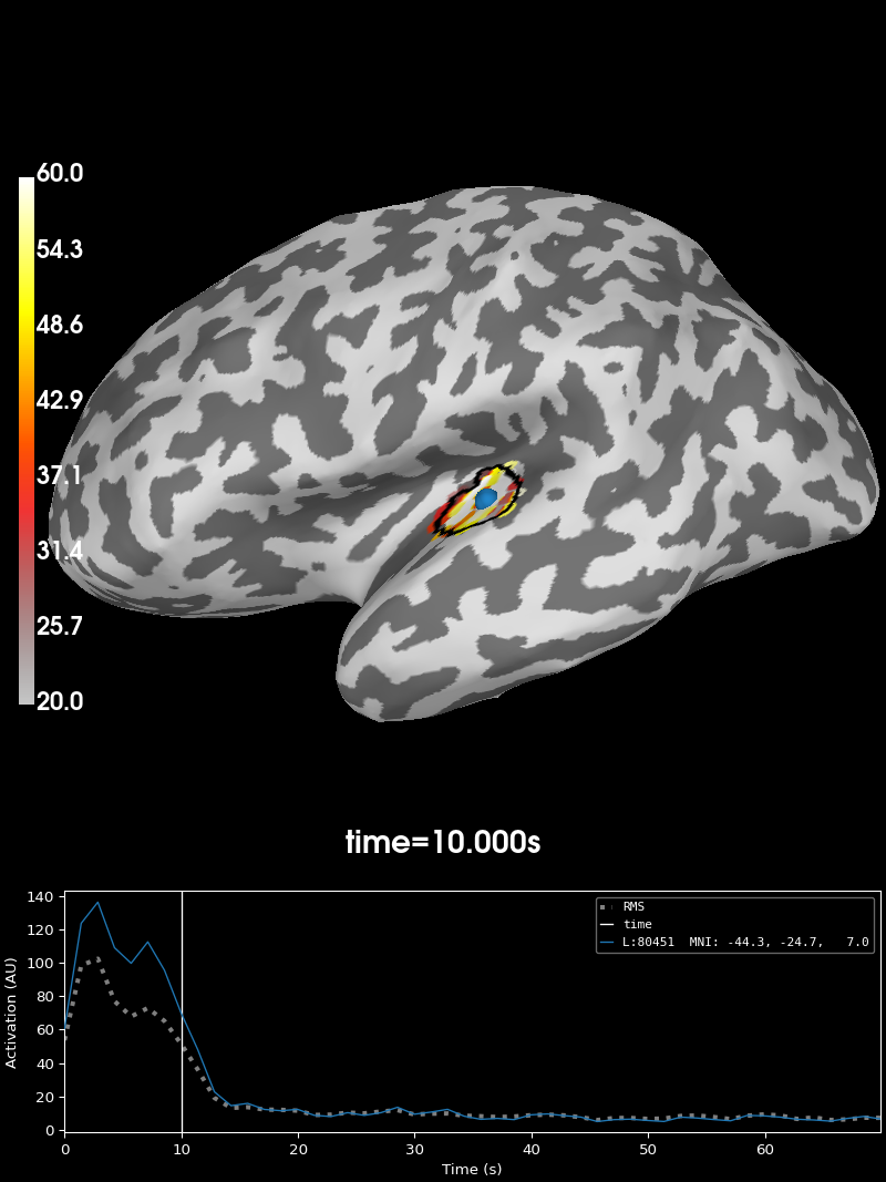
Visualize the 10 Hz PSD:
brain = stc.plot(
    initial_time=10.0,
    hemi="lh",
    views="lat",  # 10 HZ
    clim=dict(kind="value", lims=(20, 40, 60)),
    smoothing_steps=3,
    subjects_dir=subjects_dir,
)
brain.add_label(label, borders=True, color="k")

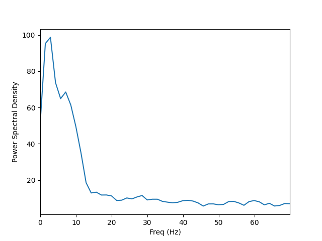
Visualize the entire spectrum:
fig, ax = plt.subplots()
ax.plot(freqs, psd_avg.mean(axis=0))
ax.set_xlabel("Freq (Hz)")
ax.set_xlim(stc.times[[0, -1]])
ax.set_ylabel("Power Spectral Density")

Total running time of the script: (0 minutes 7.589 seconds)
Estimated memory usage: 26 MB