Note
Go to the end to download the full example code.
KIT phantom dataset tutorial#
Here we read KIT data obtained from a phantom with 49 dipoles sequentially activated with 2-cycle 11 Hz sinusoidal bursts to verify source localization accuracy.
# Authors: Eric Larson <larson.eric.d@gmail.com>
#
# License: BSD-3-Clause
# Copyright the MNE-Python contributors.
import mne_bids
import numpy as np
import mne
data_path = mne.datasets.phantom_kit.data_path()
actual_pos, actual_ori = mne.dipole.get_phantom_dipoles("oyama")
actual_pos, actual_ori = actual_pos[:49], actual_ori[:49] # only 49 of 50 dipoles
bids_path = mne_bids.BIDSPath(
root=data_path,
subject="01",
task="phantom",
run="01",
datatype="meg",
)
# ignore warning about misc units
raw = mne_bids.read_raw_bids(bids_path).load_data()
# Let's apply a little bit of preprocessing (temporal filtering and reference
# regression)
picks_artifact = ["MISC 001", "MISC 002", "MISC 003"]
picks = np.r_[
mne.pick_types(raw.info, meg=True),
mne.pick_channels(raw.info["ch_names"], picks_artifact),
]
raw.filter(None, 40, picks=picks)
mne.preprocessing.regress_artifact(
raw, picks="meg", picks_artifact=picks_artifact, copy=False, proj=False
)
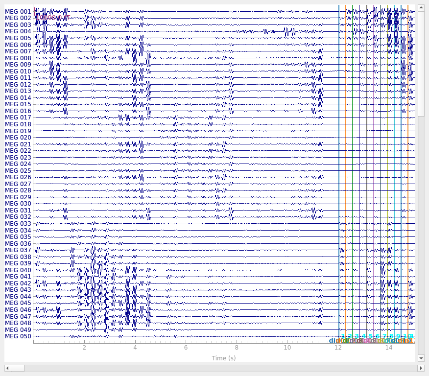
plot_scalings = dict(mag=5e-12) # large-amplitude sinusoids
raw_plot_kwargs = dict(duration=15, n_channels=50, scalings=plot_scalings)
events, event_id = mne.events_from_annotations(raw)
raw.plot(events=events, **raw_plot_kwargs)
n_dip = len(event_id)
assert n_dip == 49 # sanity check
Opening raw data file /home/circleci/mne_data/MNE-phantom-KIT-data/sub-01/meg/sub-01_task-phantom_run-01_meg.fif...
Isotrak not found
    Range : 0 ... 605800 =      0.000 ...   302.900 secs
Ready.
Reading events from /home/circleci/mne_data/MNE-phantom-KIT-data/sub-01/meg/sub-01_task-phantom_run-01_events.tsv.
Reading channel info from /home/circleci/mne_data/MNE-phantom-KIT-data/sub-01/meg/sub-01_task-phantom_run-01_channels.tsv.
Reading 0 ... 605800  =      0.000 ...   302.900 secs...
Filtering raw data in 1 contiguous segment
Setting up low-pass filter at 40 Hz

FIR filter parameters
---------------------
Designing a one-pass, zero-phase, non-causal lowpass filter:
- Windowed time-domain design (firwin) method
- Hamming window with 0.0194 passband ripple and 53 dB stopband attenuation
- Upper passband edge: 40.00 Hz
- Upper transition bandwidth: 10.00 Hz (-6 dB cutoff frequency: 45.00 Hz)
- Filter length: 661 samples (0.331 s)

[Parallel(n_jobs=1)]: Done  17 tasks      | elapsed:    0.4s
[Parallel(n_jobs=1)]: Done  71 tasks      | elapsed:    1.9s
[Parallel(n_jobs=1)]: Done 161 tasks      | elapsed:    4.9s
Used Annotations descriptions: ['dip01', 'dip02', 'dip03', 'dip04', 'dip05', 'dip06', 'dip07', 'dip08', 'dip09', 'dip10', 'dip11', 'dip12', 'dip13', 'dip14', 'dip15', 'dip16', 'dip17', 'dip18', 'dip19', 'dip20', 'dip21', 'dip22', 'dip23', 'dip24', 'dip25', 'dip26', 'dip27', 'dip28', 'dip29', 'dip30', 'dip31', 'dip32', 'dip33', 'dip34', 'dip35', 'dip36', 'dip37', 'dip38', 'dip39', 'dip40', 'dip41', 'dip42', 'dip43', 'dip44', 'dip45', 'dip46', 'dip47', 'dip48', 'dip49']
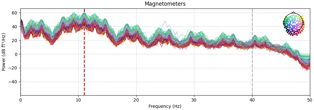
We can also look at the power spectral density to see the phantom oscillations at 11 Hz plus the expected frequency-domain sinc-like oscillations due to the time-domain boxcar windowing of the 11 Hz sinusoid.
spectrum = raw.copy().crop(0, 60).compute_psd(n_fft=10000)
fig = spectrum.plot(amplitude=False)
fig.axes[0].set_xlim(0, 50)
dip_freq = 11.0
fig.axes[0].axvline(dip_freq, color="r", ls="--", lw=2, zorder=4)
Effective window size : 5.000 (s)
Plotting power spectral density (dB=True).
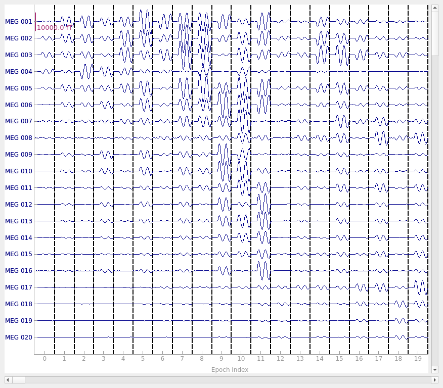
Now we can figure out our epoching parameters and epoch the data and plot it.
tmin, tmax = -0.08, 0.18
epochs = mne.Epochs(raw, tmin=tmin, tmax=tmax, decim=10, picks="data", preload=True)
del raw
epochs.plot(scalings=plot_scalings)
Used Annotations descriptions: ['dip01', 'dip02', 'dip03', 'dip04', 'dip05', 'dip06', 'dip07', 'dip08', 'dip09', 'dip10', 'dip11', 'dip12', 'dip13', 'dip14', 'dip15', 'dip16', 'dip17', 'dip18', 'dip19', 'dip20', 'dip21', 'dip22', 'dip23', 'dip24', 'dip25', 'dip26', 'dip27', 'dip28', 'dip29', 'dip30', 'dip31', 'dip32', 'dip33', 'dip34', 'dip35', 'dip36', 'dip37', 'dip38', 'dip39', 'dip40', 'dip41', 'dip42', 'dip43', 'dip44', 'dip45', 'dip46', 'dip47', 'dip48', 'dip49']
Not setting metadata
1029 matching events found
Setting baseline interval to [-0.08, 0.0] s
Applying baseline correction (mode: mean)
0 projection items activated
Using data from preloaded Raw for 1029 events and 521 original time points (prior to decimation) ...
0 bad epochs dropped
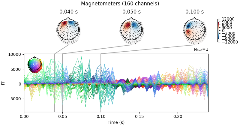
Now we can average the epochs for each dipole, get the activation at the peak time,
and create an mne.EvokedArray from the result.
No projector specified for this dataset. Please consider the method self.add_proj.
Let’s fit dipoles at each dipole’s peak activation time.
trans = mne.transforms.Transform("head", "mri", np.eye(4))
sphere = mne.make_sphere_model(r0=(0.0, 0.0, 0.0), head_radius=0.08)
cov = mne.compute_covariance(epochs, tmax=0, method="empirical")
dip, residual = mne.fit_dipole(evoked, cov, sphere, n_jobs=None)
Equiv. model fitting -> RV = 0.00364477 %
mu1 = 0.944121    lambda1 = 0.138646
mu2 = 0.665982    lambda2 = 0.684475
mu3 = -0.140083    lambda3 = -0.0127517
Set up EEG sphere model with scalp radius    80.0 mm

Reducing data rank from 160 -> 160
Estimating covariance using EMPIRICAL
Done.
Number of samples used : 17493
[done]
BEM               : <ConductorModel | Sphere (3 layers): r0=[0.0, 0.0, 0.0] R=80 mm>
MRI transform     : identity
Sphere model      : origin at (   0.00    0.00    0.00) mm, rad =    0.1 mm
Guess grid        :   20.0 mm
Guess mindist     :    5.0 mm
Guess exclude     :   20.0 mm
Using normal MEG coil definitions.
Noise covariance  : <Covariance | kind : full, shape : (160, 160), range : [-8e-28, +2.4e-26], n_samples : 17492>

Coordinate transformation: MRI (surface RAS) -> head
    1.000000 0.000000 0.000000       0.00 mm
    0.000000 1.000000 0.000000       0.00 mm
    0.000000 0.000000 1.000000       0.00 mm
    0.000000 0.000000 0.000000       1.00
Coordinate transformation: MEG device -> head
    0.998477 0.050618 -0.021924      10.00 mm
    -0.052328 0.994909 -0.086126     -15.00 mm
    0.017452 0.087142 0.996043     -88.00 mm
    0.000000 0.000000 0.000000       1.00
0 bad channels total
Read 160 MEG channels from info
105 coil definitions read
Coordinate transformation: MEG device -> head
    0.998477 0.050618 -0.021924      10.00 mm
    -0.052328 0.994909 -0.086126     -15.00 mm
    0.017452 0.087142 0.996043     -88.00 mm
    0.000000 0.000000 0.000000       1.00
MEG coil definitions created in head coordinates.
Decomposing the sensor noise covariance matrix...
Computing rank from covariance with rank=None
    Using tolerance 9.2e-16 (2.2e-16 eps * 160 dim * 0.026  max singular value)
    Estimated rank (mag): 160
    MAG: rank 160 computed from 160 data channels with 0 projectors
    Setting small MAG eigenvalues to zero (without PCA)
    Created the whitener using a noise covariance matrix with rank 160 (0 small eigenvalues omitted)

---- Computing the forward solution for the guesses...
Making a spherical guess space with radius    72.0 mm...
Filtering (grid =     20 mm)...
Surface CM = (   0.0    0.0    0.0) mm
Surface fits inside a sphere with radius   72.0 mm
Surface extent:
    x =  -72.0 ...   72.0 mm
    y =  -72.0 ...   72.0 mm
    z =  -72.0 ...   72.0 mm
Grid extent:
    x =  -80.0 ...   80.0 mm
    y =  -80.0 ...   80.0 mm
    z =  -80.0 ...   80.0 mm
729 sources before omitting any.
178 sources after omitting infeasible sources not within 20.0 - 72.0 mm.
170 sources remaining after excluding the sources outside the surface and less than    5.0 mm inside.
Go through all guess source locations...
[done 170 sources]
---- Fitted :     0.0 ms
---- Fitted :     5.0 ms
---- Fitted :    10.0 ms
---- Fitted :    15.0 ms
---- Fitted :    20.0 ms
---- Fitted :    25.0 ms
---- Fitted :    30.0 ms
---- Fitted :    35.0 ms
---- Fitted :    40.0 ms
---- Fitted :    45.0 ms
---- Fitted :    50.0 ms
---- Fitted :    55.0 ms
---- Fitted :    60.0 ms
---- Fitted :    65.0 ms
---- Fitted :    70.0 ms
---- Fitted :    75.0 ms
---- Fitted :    80.0 ms
[Parallel(n_jobs=1)]: Done  17 tasks      | elapsed:    0.7s
---- Fitted :    85.0 ms
---- Fitted :    90.0 ms
---- Fitted :    95.0 ms
---- Fitted :   100.0 ms
---- Fitted :   105.0 ms
---- Fitted :   110.0 ms
---- Fitted :   115.0 ms
---- Fitted :   120.0 ms
---- Fitted :   125.0 ms
---- Fitted :   130.0 ms
---- Fitted :   135.0 ms
---- Fitted :   140.0 ms
---- Fitted :   145.0 ms
---- Fitted :   150.0 ms
---- Fitted :   155.0 ms
---- Fitted :   160.0 ms
---- Fitted :   165.0 ms
---- Fitted :   170.0 ms
---- Fitted :   175.0 ms
---- Fitted :   180.0 ms
---- Fitted :   185.0 ms
---- Fitted :   190.0 ms
---- Fitted :   195.0 ms
---- Fitted :   200.0 ms
---- Fitted :   205.0 ms
---- Fitted :   210.0 ms
---- Fitted :   215.0 ms
---- Fitted :   220.0 ms
---- Fitted :   225.0 ms
---- Fitted :   230.0 ms
---- Fitted :   235.0 ms
---- Fitted :   240.0 ms
No projector specified for this dataset. Please consider the method self.add_proj.
49 time points fitted
Finally let’s look at the results.
print(f"Average amplitude: {np.mean(dip.amplitude) * 1e9:0.1f} nAm")
print(f"Average GOF:       {np.mean(dip.gof):0.1f}%")
diffs = 1000 * np.sqrt(np.sum((dip.pos - actual_pos) ** 2, axis=-1))
print(f"Average loc error: {np.mean(diffs):0.1f} mm")
angles = np.rad2deg(np.arccos(np.abs(np.sum(dip.ori * actual_ori, axis=1))))
print(f"Average ori error: {np.mean(angles):0.1f}°")

fig = mne.viz.plot_alignment(
    evoked.info,
    trans,
    bem=sphere,
    coord_frame="head",
    meg="helmet",
    show_axes=True,
)
fig = mne.viz.plot_dipole_locations(
    dipoles=dip, mode="arrow", color=(0.2, 1.0, 0.5), fig=fig
)

actual_amp = np.ones(len(dip))  # misc amp to create Dipole instance
actual_gof = np.ones(len(dip))  # misc GOF to create Dipole instance
dip_true = mne.Dipole(dip.times, actual_pos, actual_amp, actual_ori, actual_gof)
fig = mne.viz.plot_dipole_locations(
    dipoles=dip_true, mode="arrow", color=(0.0, 0.0, 0.0), fig=fig
)

mne.viz.set_3d_view(figure=fig, azimuth=90, elevation=90, distance=0.5)
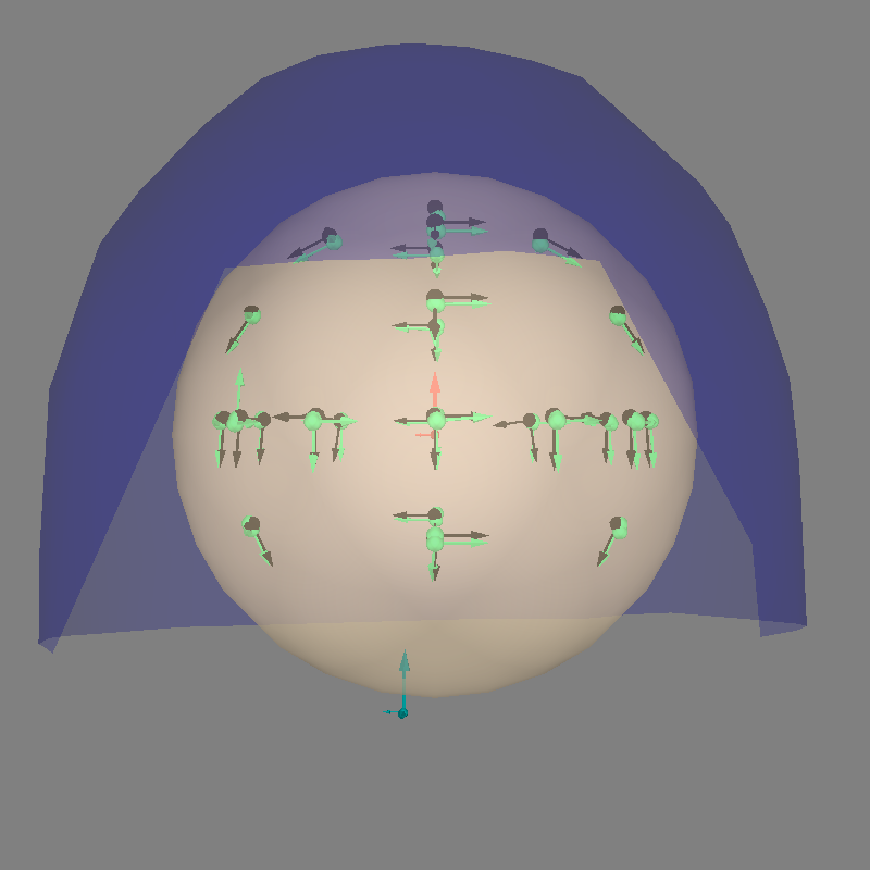
Average amplitude: 578.9 nAm
Average GOF:       99.6%
Average loc error: 1.6 mm
Average ori error: 9.6°
Getting helmet for system KIT (derived from 160 MEG channel locations)
Total running time of the script: (0 minutes 34.606 seconds)
Estimated memory usage: 1684 MB