Examples#
Examples demonstrating connectivity analysis in sensor and source space.
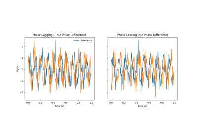
Comparing spectral connectivity computed over time or over trials
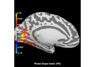
Compute Phase Slope Index (PSI) in source space for a visual stimulus
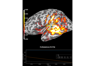
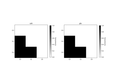
Compute coherence in source space using a MNE inverse solution
Compute connectivity using weighted symbolic mutual information (wSMI)
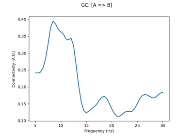
Compute directionality of connectivity with multivariate Granger causality
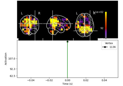
Compute envelope correlations in volume source space
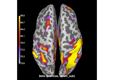
Compute full spectrum source space connectivity between labels
Compute mixed source space connectivity and visualize it using a circular graph
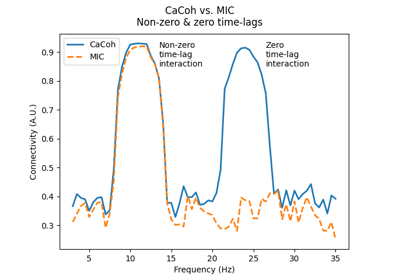
Compute multivariate measures of the imaginary part of coherency
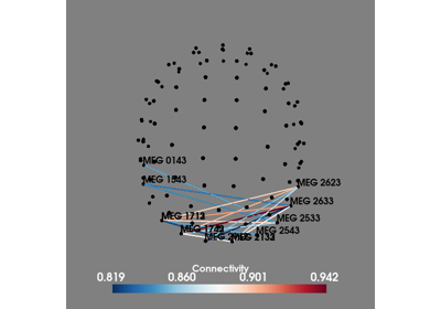
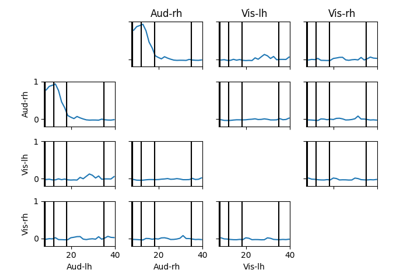
Compute seed-based time-frequency connectivity in sensor space
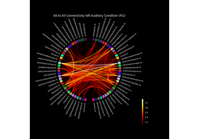
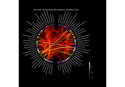
Compute source space connectivity and visualize it using a circular graph
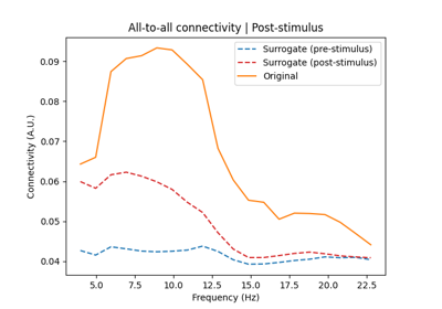
Determine the significance of connectivity estimates against baseline connectivity


Working with ragged indices for multivariate connectivity
Decoding & Decomposition Examples#
Examples demonstrating multivariate connectivity analysis using the decomposition tools of the decoding module.
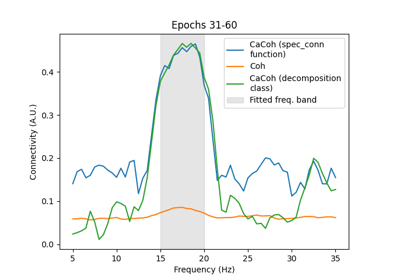
Multivariate decomposition for efficient connectivity analysis
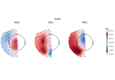
Visualising spatial contributions to multivariate connectivity
Dynamic Connectivity Examples#
Examples demonstrating connectivity analysis with dynamics. For example, this can be a vector auto-regressive model (also known as a linear dynamical system). These classes of models are generative and model the dynamics and evolution of the data.
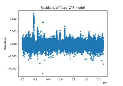
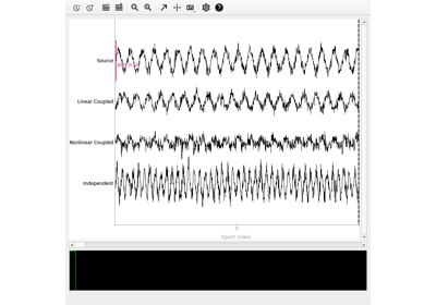
Compute vector autoregressive model (linear system)