Compute multivariate coherency/coherence

This example demonstrates how canonical coherency (CaCoh) [1] - a multivariate method based on coherency - can be used to compute connectivity between whole sets of sensors, alongside spatial patterns of the connectivity.

# Authors: Thomas S. Binns <t.s.binns@outlook.com>
#          Mohammad Orabe <orabe.mhd@gmail.com>
# License: BSD (3-clause)

import numpy as np
from matplotlib import pyplot as plt

from mne_connectivity import (
    make_signals_in_freq_bands,
    seed_target_indices,
    spectral_connectivity_epochs,
)

Background

Multivariate forms of signal analysis allow you to simultaneously consider the activity of multiple signals. In the case of connectivity, the interaction between multiple sensors can be analysed at once, producing a single connectivity spectrum. This approach brings not only practical benefits (e.g. easier interpretability of results from the dimensionality reduction), but can also offer methodological improvements (e.g. enhanced signal-to-noise ratio).

A popular bivariate measure of connectivity is coherency/coherence, which looks at the correlation between two signals in the frequency domain. However, in cases where interactions between multiple signals are of interest, computing connectivity between all possible combinations of signals leads to a very large number of results which is difficult to interpret. A common approach is to average results across these connections, however this risks reducing the signal-to-noise ratio of results and burying interactions that are present between only a small number of channels.

Canonical coherency (CaCoh) is a multivariate form of coherency that uses eigendecomposition-derived spatial filters to extract the underlying components of connectivity in a frequency-resolved manner [1]. This approach goes beyond simply aggregating information across all possible combinations of signals.

It is similar to multivariate methods based on the imaginary part of coherency (MIC & MIM [2]; see Compute multivariate measures of the imaginary part of coherency and Comparison of coherency-based methods).

Data Simulation

To demonstrate the CaCoh method, we will use some simulated data consisting of two sets of interactions between signals in a given frequency range:

• 5 seeds and 3 targets interacting in the 10-12 Hz frequency range.

• 5 seeds and 3 targets interacting in the 23-25 Hz frequency range.

We can consider the seeds and targets to be signals of different modalities, e.g. cortical EEG signals and subcortical LFP signals, cortical EEG signals and muscular EMG signals, etc…. We use the make_signals_in_freq_bands() function to simulate these signals.

# Generate simulated data
data_10_12 = make_signals_in_freq_bands(
    n_seeds=5,
    n_targets=3,
    freq_band=(10, 12),  # 10-12 Hz interaction
    rng_seed=42,
)

data_23_25 = make_signals_in_freq_bands(
    n_seeds=5,
    n_targets=3,
    freq_band=(23, 25),  # 23-25 Hz interaction
    rng_seed=44,
)

# Combine data into a single object
data = data_10_12.add_channels([data_23_25])

Setting up band-pass filter from 10 - 12 Hz

FIR filter parameters
---------------------
Designing a one-pass, zero-phase, non-causal bandpass filter:
- Windowed frequency-domain design (firwin2) method
- Hamming window
- Lower passband edge: 10.00
- Lower transition bandwidth: 1.00 Hz (-6 dB cutoff frequency: 9.50 Hz)
- Upper passband edge: 12.00 Hz
- Upper transition bandwidth: 1.00 Hz (-6 dB cutoff frequency: 12.50 Hz)
- Filter length: 661 samples (6.610 s)

Not setting metadata
10 matching events found
No baseline correction applied
0 projection items activated
Setting up band-pass filter from 23 - 25 Hz

FIR filter parameters
---------------------
Designing a one-pass, zero-phase, non-causal bandpass filter:
- Windowed frequency-domain design (firwin2) method
- Hamming window
- Lower passband edge: 23.00
- Lower transition bandwidth: 1.00 Hz (-6 dB cutoff frequency: 22.50 Hz)
- Upper passband edge: 25.00 Hz
- Upper transition bandwidth: 1.00 Hz (-6 dB cutoff frequency: 25.50 Hz)
- Filter length: 661 samples (6.610 s)

Not setting metadata
10 matching events found
No baseline correction applied
0 projection items activated

Computing CaCoh

Having simulated the signals, we can create the indices for computing connectivity between all seeds and all targets in a single multivariate connection (see Working with ragged indices for multivariate connectivity for more information), after which we compute connectivity.

For CaCoh, a set of spatial filters are found that will maximise the estimated connectivity between the seed and target signals. These maximising filters correspond to the eigenvectors with the largest eigenvalue, derived from an eigendecomposition of information from the cross-spectral density (Eq. 8 of [1]):

\(\textrm{CaCoh}=\Large{\frac{\boldsymbol{a}^T\boldsymbol{D}(\Phi) \boldsymbol{b}}{\sqrt{\boldsymbol{a}^T\boldsymbol{a}\boldsymbol{b}^T \boldsymbol{b}}}}\)

where: \(\boldsymbol{D}(\Phi)\) is the cross-spectral density between seeds and targets transformed for a given phase angle \(\Phi\); and \(\boldsymbol{a}\) and \(\boldsymbol{b}\) are eigenvectors for the seeds and targets, such that \(\boldsymbol{a}^T\boldsymbol{D}(\Phi) \boldsymbol{b}\) maximises coherency between the seeds and targets. All elements are frequency-dependent, however this is omitted for readability.

CaCoh is complex-valued in the range \([-1, 1]\) where the sign reflects the phase angle of the interaction (akin to coherency). Taking the absolute value is akin to taking the coherence, which is the magnitude of the interaction regardless of phase angle.

# Generate connectivity indices
seeds = [0, 1, 2, 3, 4, 8, 9, 10, 11, 12]
targets = [5, 6, 7, 13, 14, 15]
multivar_indices = ([seeds], [targets])

# Compute CaCoh
cacoh = spectral_connectivity_epochs(
    data, method="cacoh", indices=multivar_indices, sfreq=100, fmin=3, fmax=35
)
print(f"Results shape: {cacoh.get_data().shape} (connections x frequencies)")

# Get absolute CaCoh
cacoh_abs = np.abs(cacoh.get_data())[0]

/home/circleci/project/mne_connectivity/spectral/epochs.py:995: RuntimeWarning: There were no Annotations stored in <EpochsArray |  10 events (all good), 0 – 1.99 s, baseline off, ~270 kB, data loaded,
 '1': 10>, so metadata was not modified.
  data.add_annotations_to_metadata(overwrite=True)
Connectivity computation...
    computing connectivity for 1 connections
    using t=0.000s..1.990s for estimation (200 points)
    frequencies: 3.0Hz..35.0Hz (65 points)
Estimated data ranks:
    connection 1 - seeds (10); targets (6)
    Using multitaper spectrum estimation with 7 DPSS windows
    the following metrics will be computed: CaCoh
    computing cross-spectral density for epoch 1
    computing cross-spectral density for epoch 2
    computing cross-spectral density for epoch 3
    computing cross-spectral density for epoch 4
    computing cross-spectral density for epoch 5
    computing cross-spectral density for epoch 6
    computing cross-spectral density for epoch 7
    computing cross-spectral density for epoch 8
    computing cross-spectral density for epoch 9
    computing cross-spectral density for epoch 10
Computing CaCoh for connection 1 of 1

  0%|          | frequency blocks : 0/65 [00:00<?,       ?it/s]
  6%|▌         | frequency blocks : 4/65 [00:00<00:00,  215.05it/s]
 12%|█▏        | frequency blocks : 8/65 [00:00<00:00,  219.72it/s]
 18%|█▊        | frequency blocks : 12/65 [00:00<00:00,  218.86it/s]
 22%|██▏       | frequency blocks : 14/65 [00:00<00:00,  124.57it/s]
 28%|██▊       | frequency blocks : 18/65 [00:00<00:00,  139.81it/s]
 34%|███▍      | frequency blocks : 22/65 [00:00<00:00,  151.43it/s]
 40%|████      | frequency blocks : 26/65 [00:00<00:00,  120.94it/s]
 46%|████▌     | frequency blocks : 30/65 [00:00<00:00,  130.83it/s]
 52%|█████▏    | frequency blocks : 34/65 [00:00<00:00,  139.09it/s]
 58%|█████▊    | frequency blocks : 38/65 [00:00<00:00,  119.16it/s]
 63%|██████▎   | frequency blocks : 41/65 [00:00<00:00,  121.69it/s]
 68%|██████▊   | frequency blocks : 44/65 [00:00<00:00,  123.79it/s]
 72%|███████▏  | frequency blocks : 47/65 [00:00<00:00,  108.75it/s]
 77%|███████▋  | frequency blocks : 50/65 [00:00<00:00,  112.42it/s]
 83%|████████▎ | frequency blocks : 54/65 [00:00<00:00,  118.54it/s]
 89%|████████▉ | frequency blocks : 58/65 [00:00<00:00,  108.78it/s]
 94%|█████████▍| frequency blocks : 61/65 [00:00<00:00,  110.62it/s]
 98%|█████████▊| frequency blocks : 64/65 [00:00<00:00,  112.30it/s]
100%|██████████| frequency blocks : 65/65 [00:00<00:00,  100.40it/s]
100%|██████████| frequency blocks : 65/65 [00:00<00:00,  107.27it/s]
[Connectivity computation done]
Results shape: (1, 65) (connections x frequencies)

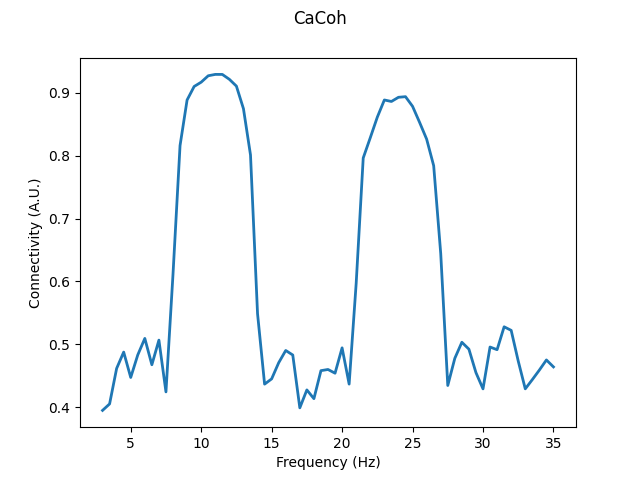
As you can see below, using CaCoh we have summarised the most relevant connectivity information from our 10 seed channels and 6 target channels as a single spectrum of connectivity values. This lower-dimensional representation of signal interactions is much more interpretable when analysing connectivity in complex systems such as the brain.

# Plot CaCoh
fig, axis = plt.subplots(1, 1)
axis.plot(cacoh.freqs, cacoh_abs, linewidth=2)
axis.set_xlabel("Frequency (Hz)")
axis.set_ylabel("Connectivity (A.U.)")
fig.suptitle("CaCoh")

Text(0.5, 0.98, 'CaCoh')

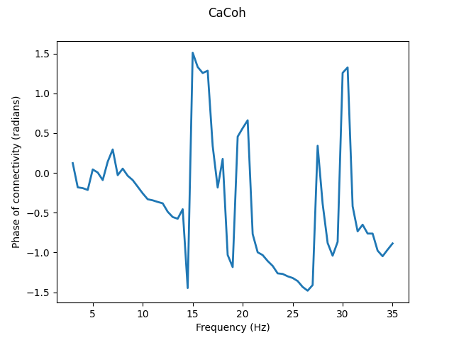
Note that we plot the absolute values of the results (coherence) rather than the complex values (coherency). The absolute value of connectivity will generally be of most interest. However, information such as the phase of interaction can only be extracted from the complex-valued results, e.g. with the numpy.angle() function.

# Plot phase of connectivity
fig, axis = plt.subplots(1, 1)
axis.plot(cacoh.freqs, np.angle(cacoh.get_data()[0]), linewidth=2)
axis.set_xlabel("Frequency (Hz)")
axis.set_ylabel("Phase of connectivity (radians)")
fig.suptitle("CaCoh")

Text(0.5, 0.98, 'CaCoh')

CaCoh versus coherence

To further demonstrate the signal-to-noise ratio benefits of CaCoh, below we compute connectivity between each seed and target using bivariate coherence. With our 10 seeds and 6 targets, this gives us a total of 60 unique connections which is very difficult to interpret without aggregating some information. A common approach is to simply average across these connections, which we do below.

# Define bivariate connectivity indices
bivar_indices = seed_target_indices(seeds, targets)

# Compute bivariate coherence
coh = spectral_connectivity_epochs(
    data, method="coh", indices=bivar_indices, sfreq=100, fmin=3, fmax=35
)
print(f"Original results shape: {coh.get_data().shape} (connections x frequencies)")

# Average results across connections
coh_mean = np.mean(coh.get_data(), axis=0)
print(f"Averaged results shape: {coh_mean.shape} (connections x frequencies)")

/home/circleci/project/mne_connectivity/spectral/epochs.py:995: RuntimeWarning: There were no Annotations stored in <EpochsArray |  10 events (all good), 0 – 1.99 s, baseline off, ~270 kB, data loaded,
 '1': 10>, so metadata was not modified.
  data.add_annotations_to_metadata(overwrite=True)
Connectivity computation...
    computing connectivity for 60 connections
    using t=0.000s..1.990s for estimation (200 points)
    frequencies: 3.0Hz..35.0Hz (65 points)
    Using multitaper spectrum estimation with 7 DPSS windows
    the following metrics will be computed: Coherence
    computing cross-spectral density for epoch 1
    computing cross-spectral density for epoch 2
    computing cross-spectral density for epoch 3
    computing cross-spectral density for epoch 4
    computing cross-spectral density for epoch 5
    computing cross-spectral density for epoch 6
    computing cross-spectral density for epoch 7
    computing cross-spectral density for epoch 8
    computing cross-spectral density for epoch 9
    computing cross-spectral density for epoch 10
[Connectivity computation done]
Original results shape: (60, 65) (connections x frequencies)
Averaged results shape: (65,) (connections x frequencies)

Plotting the bivariate and multivariate results together, we can see that coherence still captures the interactions at 10-12 Hz and 23-25 Hz, however the scale of the connectivity is much smaller. This reflects the fact that CaCoh is able to capture the relevant components of interactions between multiple signals, regardless of whether they are present in all channels.

# Plot CaCoh & Coh
fig, axis = plt.subplots(1, 1)
axis.plot(cacoh.freqs, cacoh_abs - np.min(cacoh_abs), linewidth=2, label="CaCoh")
axis.plot(coh.freqs, coh_mean - np.min(coh_mean), linewidth=2, label="Coh")
axis.set_xlabel("Frequency (Hz)")
axis.set_ylabel("Baseline-corrected connectivity (A.U.)")
axis.legend()
fig.suptitle("CaCoh vs. coherence")

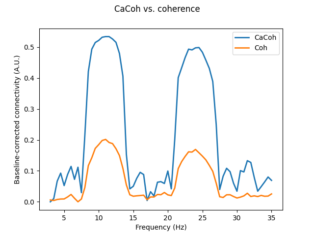
Text(0.5, 0.98, 'CaCoh vs. coherence')

The ability of multivariate connectivity methods to capture the underlying components of connectivity is extremely useful when dealing with data from a large number of channels, with inter-channel interactions at distinct frequencies, a problem explored in more detail in the Compute multivariate measures of the imaginary part of coherency example.

Extracting spatial information from CaCoh

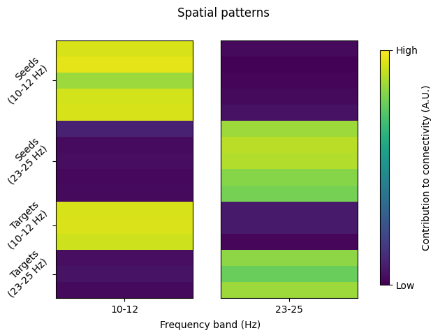
Whilst a lower-dimensional representation of connectivity information is useful, we lose information about which channels are involved in the connectivity. Thankfully, this information can be recovered by constructing spatial patterns of connectivity from the spatial filters [3].

The spatial patterns are stored under attrs['patterns'] of the connectivity class, with one value per frequency for each channel in the seeds and targets. The patterns can be positive- and negative-valued. Sign differences of the patterns can be used to visualise the orientation of underlying dipole sources, whereas their absolute value reflects the strength of a channel’s contribution to the connectivity component. The spatial patterns are not bound between \([-1, 1]\).

Averaging across the patterns in the 10-12 Hz and 23-25 Hz ranges, we can see how it is possible to identify which channels are contributing to connectivity at different frequencies.

freqs = cacoh.freqs
fbands = ((10, 12), ((23, 25)))

fig, axes = plt.subplots(1, 2)

# patterns have shape [seeds/targets x cons x channels x freqs (x times)]
patterns = np.abs(np.array(cacoh.attrs["patterns"]))
seed_pattern = patterns[0, :, : len(seeds)]
target_pattern = patterns[1, :, : len(targets)]

vmin = np.nanmin(patterns)
vmax = np.nanmax(patterns)

for axis, fband in zip(axes, fbands):
    # average across frequencies
    seed_pattern_fband = np.mean(
        seed_pattern[0, :, freqs.index(fband[0]) : freqs.index(fband[1]) + 1], axis=1
    )
    target_pattern_fband = np.mean(
        target_pattern[0, :, freqs.index(fband[0]) : freqs.index(fband[1]) + 1], axis=1
    )

    # combine into a single array
    pattern_fband = np.concatenate((seed_pattern_fband, target_pattern_fband), axis=0)

    # plot the pattern
    mesh = axis.pcolormesh(
        np.flip(np.expand_dims(pattern_fband, 1)), vmin=vmin, vmax=vmax
    )
    axis.set_yticks([1.5, 4.5, 8.5, 13.5])
    axis.set_xticks([0.5])
    axis.set_xticklabels([f"{fband[0]}-{fband[1]}"])

# Label axes
fig.suptitle("Spatial patterns")
axes[0].set_yticklabels(
    [
        "Targets\n(23-25 Hz)",
        "Targets\n(10-12 Hz)",
        "Seeds\n(23-25 Hz)",
        "Seeds\n(10-12 Hz)",
    ],
    rotation=45,
    va="center",
)
axes[0].set_ylabel("Channels")
axes[1].get_yaxis().set_visible(False)
fig.text(0.47, 0.02, "Frequency band (Hz)", ha="center")

# Set colourbar
fig.subplots_adjust(right=0.8)
cbar_axis = fig.add_axes([0.85, 0.15, 0.02, 0.7])
fig.colorbar(mesh, cax=cbar_axis)
cbar_axis.set_ylabel("Contribution to connectivity (A.U.)")
cbar_axis.set_yticks([vmin, vmax])
cbar_axis.set_yticklabels(["Low", "High"])

plt.show()

For an example on interpreting spatial filters with real data, see the Compute multivariate measures of the imaginary part of coherency example.

Handling high-dimensional data

An important issue to consider when using these multivariate methods is overfitting, which risks biasing connectivity estimates to maximise noise in the data. This risk can be reduced by performing a preliminary dimensionality reduction prior to estimating the connectivity with a singular value decomposition (Eq. 15 of [1]). The degree of this dimensionality reduction can be specified using the rank argument, which by default will not perform any dimensionality reduction (assuming your data is full rank; see below if not). Choosing an expected rank of the data requires a priori knowledge about the number of components you expect to observe in the data.

When comparing CaCoh scores across recordings, it is highly recommended to estimate connectivity from the same number of channels (or equally from the same degree of rank subspace projection) to avoid biases in connectivity estimates. Bias can be avoided by specifying a consistent rank subspace to project to using the rank argument, standardising your connectivity estimates regardless of changes in e.g. the number of channels across recordings. Note that this does not refer to the number of seeds and targets within a connection being identical, rather to the number of seeds and targets across connections.

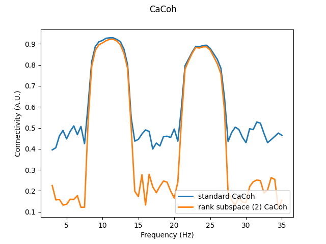
Here, we project our seed and target data to only the first 2 components of our rank subspace. Results show that the general spectral pattern of connectivity is retained in the rank subspace-projected data, suggesting that a fair degree of redundant connectivity information is contained in the excluded components of the seed and target data.

We also assert that the spatial patterns of MIC are returned in the original sensor space despite this rank subspace projection, being reconstructed using the products of the singular value decomposition (Eqs. 46 & 47 of [2]).

# Compute CaCoh following rank subspace projection
cacoh_red = spectral_connectivity_epochs(
    data,
    method="cacoh",
    indices=multivar_indices,
    sfreq=100,
    fmin=3,
    fmax=35,
    rank=([2], [2]),
)

# compare standard and rank subspace-projected CaCoh
fig, axis = plt.subplots(1, 1)
axis.plot(cacoh.freqs, np.abs(cacoh.get_data()[0]), linewidth=2, label="standard CaCoh")
axis.plot(
    cacoh_red.freqs,
    np.abs(cacoh_red.get_data()[0]),
    linewidth=2,
    label="rank subspace (2) CaCoh",
)
axis.set_xlabel("Frequency (Hz)")
axis.set_ylabel("Connectivity (A.U.)")
axis.legend(loc="lower right")
fig.suptitle("CaCoh")

# no. channels equal with and without projecting to rank subspace for patterns
assert patterns[0, 0].shape[0] == np.array(cacoh_red.attrs["patterns"])[0, 0].shape[0]
assert patterns[1, 0].shape[0] == np.array(cacoh_red.attrs["patterns"])[1, 0].shape[0]

/home/circleci/project/mne_connectivity/spectral/epochs.py:995: RuntimeWarning: There were no Annotations stored in <EpochsArray |  10 events (all good), 0 – 1.99 s, baseline off, ~270 kB, data loaded,
 '1': 10>, so metadata was not modified.
  data.add_annotations_to_metadata(overwrite=True)
Connectivity computation...
    computing connectivity for 1 connections
    using t=0.000s..1.990s for estimation (200 points)
    frequencies: 3.0Hz..35.0Hz (65 points)
    Using multitaper spectrum estimation with 7 DPSS windows
    the following metrics will be computed: CaCoh
    computing cross-spectral density for epoch 1
    computing cross-spectral density for epoch 2
    computing cross-spectral density for epoch 3
    computing cross-spectral density for epoch 4
    computing cross-spectral density for epoch 5
    computing cross-spectral density for epoch 6
    computing cross-spectral density for epoch 7
    computing cross-spectral density for epoch 8
    computing cross-spectral density for epoch 9
    computing cross-spectral density for epoch 10
Computing CaCoh for connection 1 of 1

  0%|          | frequency blocks : 0/65 [00:00<?,       ?it/s]
 18%|█▊        | frequency blocks : 12/65 [00:00<00:00,  691.74it/s]
 37%|███▋      | frequency blocks : 24/65 [00:00<00:00,  704.92it/s]
 55%|█████▌    | frequency blocks : 36/65 [00:00<00:00,  702.91it/s]
 74%|███████▍  | frequency blocks : 48/65 [00:00<00:00,  705.71it/s]
 92%|█████████▏| frequency blocks : 60/65 [00:00<00:00,  705.00it/s]
100%|██████████| frequency blocks : 65/65 [00:00<00:00,  702.84it/s]
[Connectivity computation done]

See Compute multivariate measures of the imaginary part of coherency for an example of applying the rank subspace projection to real data with a large number of channels.

In the case that your data is not full rank and rank is left as None, an automatic rank computation is performed and an appropriate degree of dimensionality reduction will be enforced. The rank of the data is determined by computing the singular values of the data and finding those within a factor of \(1e^{-6}\) relative to the largest singular value.

Whilst unlikely, there may be scenarios in which this threshold may be too lenient. In these cases, you should inspect the singular values of your data to identify an appropriate degree of dimensionality reduction to perform, which you can then specify manually using the rank argument. The code below shows one possible approach for finding an appropriate rank of close-to-singular data with a more conservative threshold.

# gets the singular values of the data across epochs
s = np.linalg.svd(data, compute_uv=False).min(axis=0)
# finds how many singular values are 'close' to the largest singular value
rank = np.count_nonzero(s >= s[0] * 1e-4)  # 1e-4 is the 'closeness' criteria, which is
# a hyper-parameter

Limitations

Multivariate methods offer many benefits in the form of dimensionality reduction and signal-to-noise ratio improvements. However, no method is perfect. When we simulated the data, we mentioned how we considered the seeds and targets to be signals of different modalities. This is an important factor in whether CaCoh should be used over methods based solely on the imaginary part of coherency such as MIC and MIM.

In short, if you want to examine connectivity between signals from the same modality, you should consider using another method instead of CaCoh. Rather, methods based on the imaginary part of coherency such as MIC and MIM should be used to avoid spurious connectivity estimates stemming from e.g. volume conduction artefacts.

On the other hand, if you want to examine connectivity between signals from different modalities, CaCoh is a more appropriate method than MIC/MIM. This is because volume conduction artefacts are of less concern, and CaCoh does not risk biasing connectivity estimates towards interactions with particular phase lags like MIC/MIM.

These scenarios are described in more detail in the Comparison of coherency-based methods example.

References

[1] (1,2,3,4)

Carmen Vidaurre, Guido Nolte, Ingmar E.J. de Vries, M. Gómez, Tjeerd W. Boonstra, K.-R. Müller, Arno Villringer, and Vadim V. Nikulin. Canonical maximization of coherence: a novel tool for investigation of neuronal interactions between two datasets. NeuroImage, 201:116009, 2019. doi:10.1016/j.neuroimage.2019.116009.

[2] (1,2)

Arne Ewald, Laura Marzetti, Filippo Zappasodi, Frank C. Meinecke, and Guido Nolte. Estimating true brain connectivity from EEG/MEG data invariant to linear and static transformations in sensor space. NeuroImage, 60(1):476–488, 2012. doi:10.1016/j.neuroimage.2011.11.084.

[3]

Stefan Haufe, Frank Meinecke, Kai Görgen, Sven Dähne, John-Dylan Haynes, Benjamin Blankertz, and Felix Bießmann. On the interpretation of weight vectors of linear models in multivariate neuroimaging. NeuroImage, 87:96–110, 2014. doi:10.1016/j.neuroimage.2013.10.067.