Determine the significance of connectivity estimates against baseline connectivity

This example demonstrates how surrogate data can be generated to assess whether connectivity estimates are significantly greater than baseline.

# Author: Thomas S. Binns <t.s.binns@outlook.com>
# License: BSD (3-clause)
# sphinx_gallery_thumbnail_number = 3

import matplotlib.pyplot as plt
import mne
import numpy as np
from mne.datasets import somato

from mne_connectivity import (
    make_surrogate_evoked_data,
    make_surrogate_resting_data,
    spectral_connectivity_epochs,
)

Background

When performing connectivity analyses, we often want to know whether the results we observe reflect genuine interactions between signals. We can assess this by performing statistical tests between our connectivity estimates and a ‘baseline’ level of connectivity. However, due to factors such as background noise and sample size-dependent biases (see e.g., Vinck et al.[1]), it is often not appropriate to treat 0 as this baseline. Therefore, we need a way to estimate the baseline level of connectivity.

One approach is to manipulate the original data in such a way that the covariance structure is destroyed, creating surrogate data. Connectivity estimates from the original and surrogate data can then be compared to determine whether the original data contains significant interactions.

Such surrogate data can be easily generated in MNE-Connectivity using the make_surrogate_resting_data() [2] and make_surrogate_evoked_data() [3] functions. In this example, we will demonstrate how surrogate data can be created, and how you can use this to assess the statistical significance of your connectivity estimates.

Loading the data

We start by loading from the Somatosensory dataset, MEG data showing event-related activity in response to somatosensory stimuli. We construct epochs around these events in the time window [-1.5, 1.0] seconds.

# Load data
data_path = somato.data_path()
raw_fname = data_path / "sub-01" / "meg" / "sub-01_task-somato_meg.fif"
raw = mne.io.read_raw_fif(raw_fname)
events = mne.find_events(raw, stim_channel="STI 014")

# Pre-processing
raw.pick("grad").load_data()  # focus on gradiometers
raw.filter(1, 35)
raw, events = raw.resample(sfreq=100, events=events)  # reduce compute time

# Construct epochs around events
epochs = mne.Epochs(
    raw, events, event_id=1, tmin=-1.5, tmax=1.0, baseline=(-0.5, 0), preload=True
)
epochs = epochs[:30]  # select a subset of epochs to speed up computation

Opening raw data file /home/circleci/mne_data/MNE-somato-data/sub-01/meg/sub-01_task-somato_meg.fif...
    Range : 237600 ... 506999 =    791.189 ...  1688.266 secs
Ready.
Finding events on: STI 014
111 events found on stim channel STI 014
Event IDs: [1]
Reading 0 ... 269399  =      0.000 ...   897.077 secs...
Filtering raw data in 1 contiguous segment
Setting up band-pass filter from 1 - 35 Hz

FIR filter parameters
---------------------
Designing a one-pass, zero-phase, non-causal bandpass filter:
- Windowed time-domain design (firwin) method
- Hamming window with 0.0194 passband ripple and 53 dB stopband attenuation
- Lower passband edge: 1.00
- Lower transition bandwidth: 1.00 Hz (-6 dB cutoff frequency: 0.50 Hz)
- Upper passband edge: 35.00 Hz
- Upper transition bandwidth: 8.75 Hz (-6 dB cutoff frequency: 39.38 Hz)
- Filter length: 993 samples (3.307 s)

Not setting metadata
111 matching events found
Applying baseline correction (mode: mean)
0 projection items activated
Using data from preloaded Raw for 111 events and 251 original time points ...
0 bad epochs dropped

Assessing connectivity in non-evoked data

We will first demonstrate how connectivity can be assessed from non-evoked data. In this example, we use data from the pre-trial period of [-1.5, -0.5] seconds. We compute time-resolved Fourier coefficients of the data using the compute_tfr() method with output="complex".

Next, we pass these coefficients to spectral_connectivity_epochs() to compute connectivity using the imaginary part of coherency (imcoh). Our indices specify that connectivity between all unique pairs of channels should be computed.

# Compute time-resolved Fourier coefficients for pre-trial data
freqs = np.arange(4, 23, 2)  # take every other frequency to reduce compute time
tfr_kwargs = dict(
    freqs=freqs,
    n_cycles=freqs / 2.0,
    method="morlet",
    decim=3,  # decimate in time-domain to reduce compute time
    output="complex",
    n_jobs=1,
)
pretrial_coeffs = epochs.compute_tfr(tmin=None, tmax=-0.5, **tfr_kwargs)

# Compute connectivity for pre-trial data
indices = np.tril_indices(epochs.info["nchan"], k=-1)  # all unique connections
pretrial_con = spectral_connectivity_epochs(
    pretrial_coeffs, method="imcoh", indices=indices
)
pretrial_con = np.abs(pretrial_con.get_data()).mean(
    axis=(0, 2)  # average connections and timepoints
)

Connectivity computation...
    using t=-1.500s..-0.510s for estimation (34 points)
    frequencies: 4.0Hz..22.0Hz (10 points)
    computing connectivity for 20706 connections
    the following metrics will be computed: Imaginary Coherence
    computing cross-spectral density for epoch 1
    computing cross-spectral density for epoch 2
    computing cross-spectral density for epoch 3
    computing cross-spectral density for epoch 4
    computing cross-spectral density for epoch 5
    computing cross-spectral density for epoch 6
    computing cross-spectral density for epoch 7
    computing cross-spectral density for epoch 8
    computing cross-spectral density for epoch 9
    computing cross-spectral density for epoch 10
    computing cross-spectral density for epoch 11
    computing cross-spectral density for epoch 12
    computing cross-spectral density for epoch 13
    computing cross-spectral density for epoch 14
    computing cross-spectral density for epoch 15
    computing cross-spectral density for epoch 16
    computing cross-spectral density for epoch 17
    computing cross-spectral density for epoch 18
    computing cross-spectral density for epoch 19
    computing cross-spectral density for epoch 20
    computing cross-spectral density for epoch 21
    computing cross-spectral density for epoch 22
    computing cross-spectral density for epoch 23
    computing cross-spectral density for epoch 24
    computing cross-spectral density for epoch 25
    computing cross-spectral density for epoch 26
    computing cross-spectral density for epoch 27
    computing cross-spectral density for epoch 28
    computing cross-spectral density for epoch 29
    computing cross-spectral density for epoch 30
[Connectivity computation done]

Next, we generate the surrogate data by passing the coefficients into the make_surrogate_resting_data() function. This approach destroys the data’s covariance structure by randomly shuffling the order of epochs, independently for each channel. To get a reliable estimate of the baseline connectivity, we perform this shuffling procedure n_shuffle times, producing n_shuffle surrogate datasets. We can then iterate over these shuffles and compute the connectivity for each one.

# Generate pre-trial surrogate data
n_shuffles = 100  # recommended is ≥ 1,000; limited here to reduce compute time
pretrial_surrogates = make_surrogate_resting_data(
    pretrial_coeffs, n_shuffles=n_shuffles, rng_seed=42
)

# Compute connectivity for pre-trial surrogate data
pretrial_surrogate_con = []
for shuffle_i, surrogate in enumerate(pretrial_surrogates, 1):
    print(f"Computing connectivity for shuffle {shuffle_i} of {n_shuffles}")
    surrogate_con = spectral_connectivity_epochs(
        surrogate, method="imcoh", indices=indices, verbose=False
    )
    pretrial_surrogate_con.append(
        np.abs(surrogate_con.get_data()).mean(axis=(0, 2))
    )  # average connections and timepoints
pretrial_surrogate_con = np.array(pretrial_surrogate_con)

Computing connectivity for shuffle 1 of 100
Computing connectivity for shuffle 2 of 100
Computing connectivity for shuffle 3 of 100
Computing connectivity for shuffle 4 of 100
Computing connectivity for shuffle 5 of 100
Computing connectivity for shuffle 6 of 100
Computing connectivity for shuffle 7 of 100
Computing connectivity for shuffle 8 of 100
Computing connectivity for shuffle 9 of 100
Computing connectivity for shuffle 10 of 100
Computing connectivity for shuffle 11 of 100
Computing connectivity for shuffle 12 of 100
Computing connectivity for shuffle 13 of 100
Computing connectivity for shuffle 14 of 100
Computing connectivity for shuffle 15 of 100
Computing connectivity for shuffle 16 of 100
Computing connectivity for shuffle 17 of 100
Computing connectivity for shuffle 18 of 100
Computing connectivity for shuffle 19 of 100
Computing connectivity for shuffle 20 of 100
Computing connectivity for shuffle 21 of 100
Computing connectivity for shuffle 22 of 100
Computing connectivity for shuffle 23 of 100
Computing connectivity for shuffle 24 of 100
Computing connectivity for shuffle 25 of 100
Computing connectivity for shuffle 26 of 100
Computing connectivity for shuffle 27 of 100
Computing connectivity for shuffle 28 of 100
Computing connectivity for shuffle 29 of 100
Computing connectivity for shuffle 30 of 100
Computing connectivity for shuffle 31 of 100
Computing connectivity for shuffle 32 of 100
Computing connectivity for shuffle 33 of 100
Computing connectivity for shuffle 34 of 100
Computing connectivity for shuffle 35 of 100
Computing connectivity for shuffle 36 of 100
Computing connectivity for shuffle 37 of 100
Computing connectivity for shuffle 38 of 100
Computing connectivity for shuffle 39 of 100
Computing connectivity for shuffle 40 of 100
Computing connectivity for shuffle 41 of 100
Computing connectivity for shuffle 42 of 100
Computing connectivity for shuffle 43 of 100
Computing connectivity for shuffle 44 of 100
Computing connectivity for shuffle 45 of 100
Computing connectivity for shuffle 46 of 100
Computing connectivity for shuffle 47 of 100
Computing connectivity for shuffle 48 of 100
Computing connectivity for shuffle 49 of 100
Computing connectivity for shuffle 50 of 100
Computing connectivity for shuffle 51 of 100
Computing connectivity for shuffle 52 of 100
Computing connectivity for shuffle 53 of 100
Computing connectivity for shuffle 54 of 100
Computing connectivity for shuffle 55 of 100
Computing connectivity for shuffle 56 of 100
Computing connectivity for shuffle 57 of 100
Computing connectivity for shuffle 58 of 100
Computing connectivity for shuffle 59 of 100
Computing connectivity for shuffle 60 of 100
Computing connectivity for shuffle 61 of 100
Computing connectivity for shuffle 62 of 100
Computing connectivity for shuffle 63 of 100
Computing connectivity for shuffle 64 of 100
Computing connectivity for shuffle 65 of 100
Computing connectivity for shuffle 66 of 100
Computing connectivity for shuffle 67 of 100
Computing connectivity for shuffle 68 of 100
Computing connectivity for shuffle 69 of 100
Computing connectivity for shuffle 70 of 100
Computing connectivity for shuffle 71 of 100
Computing connectivity for shuffle 72 of 100
Computing connectivity for shuffle 73 of 100
Computing connectivity for shuffle 74 of 100
Computing connectivity for shuffle 75 of 100
Computing connectivity for shuffle 76 of 100
Computing connectivity for shuffle 77 of 100
Computing connectivity for shuffle 78 of 100
Computing connectivity for shuffle 79 of 100
Computing connectivity for shuffle 80 of 100
Computing connectivity for shuffle 81 of 100
Computing connectivity for shuffle 82 of 100
Computing connectivity for shuffle 83 of 100
Computing connectivity for shuffle 84 of 100
Computing connectivity for shuffle 85 of 100
Computing connectivity for shuffle 86 of 100
Computing connectivity for shuffle 87 of 100
Computing connectivity for shuffle 88 of 100
Computing connectivity for shuffle 89 of 100
Computing connectivity for shuffle 90 of 100
Computing connectivity for shuffle 91 of 100
Computing connectivity for shuffle 92 of 100
Computing connectivity for shuffle 93 of 100
Computing connectivity for shuffle 94 of 100
Computing connectivity for shuffle 95 of 100
Computing connectivity for shuffle 96 of 100
Computing connectivity for shuffle 97 of 100
Computing connectivity for shuffle 98 of 100
Computing connectivity for shuffle 99 of 100
Computing connectivity for shuffle 100 of 100

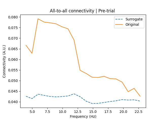
We can plot the connectivity of the pre-trial data against the surrogate data, averaged over all shuffles. This shows a strong degree of coupling in the alpha band (~8-12 Hz), with weaker coupling in the lower range of the beta band (~13-20 Hz). A simple visual inspection shows that connectivity in the alpha and beta bands are above the baseline level of connectivity estimated from the surrogate data. However, we need to confirm this statistically.

# Plot pre-trial actual vs. surrogate connectivity
fig, ax = plt.subplots(1, 1)
ax.plot(freqs, pretrial_surrogate_con.mean(axis=0), linestyle="--", label="Surrogate")
ax.plot(freqs, pretrial_con, label="Original")
ax.set_xlabel("Frequency (Hz)")
ax.set_ylabel("Connectivity (A.U.)")
ax.set_title("All-to-all connectivity | Pre-trial ")
ax.legend()

<matplotlib.legend.Legend object at 0x763d9357b4d0>

Assessing the statistical significance of our connectivity estimates can be done with the following simple procedure [2]

\(p=\LARGE{\frac{\Sigma_{s=1}^Sc_s}{S}}\) ,

\begin{flalign*} c_s = \begin{cases} 1 & \text{if }\text{Con}\leq\text{Con}_{\text{s}} \\ 0 & \text{otherwise} \end{cases} , && \end{flalign*}

where: \(p\) is our p-value; \(s\) is a given shuffle iteration of \(S\) total shuffles; and \(c\) is a binary indicator of whether the true connectivity, \(\text{Con}\), is greater than the surrogate connectivity, \(\text{Con}_{\text{s}}\), for a given shuffle.

Note that for connectivity methods which produce negative scores (e.g., imaginary part of coherency, time-reversed Granger causality, etc…), you should take the absolute values before testing. Similar adjustments should be made for methods that produce scores centred around non-zero values (e.g., 0.5 for directed phase lag index).

Below, we determine the statistical significance of connectivity in the lower beta band. We simplify this by averaging over all connections and corresponding frequency bins. We could of course also test the significance of each connection, each frequency bin, or other frequency bands such as the alpha band. Naturally, any tests involving multiple connections, frequencies, and/or times should be corrected for multiple comparisons.

The test confirms our visual inspection, showing that connectivity in the lower beta band is significantly above the baseline level of connectivity at an alpha of 0.05, which we can take as evidence of genuine interactions in this frequency band.

# Find indices of lower beta frequencies
beta_freqs = np.where((freqs >= 13) & (freqs <= 20))[0]

# Compute lower beta connectivity for pre-trial data
beta_con_pretrial = pretrial_con[beta_freqs].mean()

# Compute lower beta connectivity for surrogate data
beta_con_pretrial_surrogate = pretrial_surrogate_con[:, beta_freqs].mean(axis=1)

# Compute p-value for pre-trial lower beta coupling
p_val = np.sum(beta_con_pretrial <= beta_con_pretrial_surrogate) / n_shuffles
print(f"p = {p_val:.2f}")

p = 0.00

Assessing connectivity in evoked data

When generating surrogate data, it is important to distinguish non-evoked data (e.g., resting-state, pre/inter-trial data) from evoked data (where a stimulus is presented or an action performed at a set time during each epoch). Critically, evoked data contains a temporal structure that is consistent across epochs. Shuffling these epochs across channels (as is done in make_surrogate_resting_data()) will fail to adequately disrupt the covariance structure.

Any connectivity estimates will therefore overestimate the baseline connectivity in your data, increasing the likelihood of type II errors (see the Notes section of make_surrogate_resting_data() for more information, and see the section Generating surrogate connectivity from inappropriate data for a demonstration).

In cases where you want to assess connectivity in evoked data, you can use the alternative make_surrogate_evoked_data() function. This approach involves cutting the time series at a random point and reversing the cut portion, independently for each epoch and channel.

Supported data types

While make_surrogate_resting_data() supports Epochs, EpochsSpectrum, and EpochsTFR objects, make_surrogate_evoked_data() data does not support EpochsSpectrum objects, as there is no time dimension to manipulate.

If you want to compare the significance of connectivity estimates for evoked data derived from an EpochsSpectrum object, you can first generate surrogates from the Epochs data, and then compute the EpochsSpectrum representations from these.

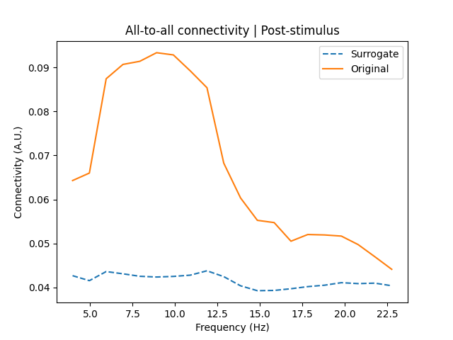
Again, there is pronounced alpha coupling (stronger than in the pre-trial data) and weaker beta coupling, both of which appear to be above the baseline level of connectivity.

# Compute time-resolved Fourier coefficients for post-stimulus data
poststim_coeffs = epochs.compute_tfr(tmin=0.0, tmax=None, **tfr_kwargs)

# Compute connectivity for post-stimulus data
poststim_con = spectral_connectivity_epochs(
    poststim_coeffs, method="imcoh", indices=indices, verbose=False
)
poststim_con = np.abs(poststim_con.get_data()).mean(
    axis=(0, 2)  # average connections and timepoints
)

# Generate post-stimulus surrogate data
poststim_surrogates = make_surrogate_evoked_data(
    poststim_coeffs, n_shuffles=n_shuffles, rng_seed=42
)

# Compute connectivity for post-stimulus surrogate data
poststim_surrogate_con = []
for shuffle_i, surrogate in enumerate(poststim_surrogates, 1):
    print(f"Computing connectivity for shuffle {shuffle_i} of {n_shuffles}")
    surrogate_con = spectral_connectivity_epochs(
        surrogate, method="imcoh", indices=indices, verbose=False
    )
    poststim_surrogate_con.append(
        np.abs(surrogate_con.get_data()).mean(axis=(0, 2))
    )  # average connections and timepoints
poststim_surrogate_con = np.array(poststim_surrogate_con)

# Plot post-stimulus actual vs. surrogate connectivity
fig, ax = plt.subplots(1, 1)
ax.plot(freqs, poststim_surrogate_con.mean(axis=0), linestyle="--", label="Surrogate")
ax.plot(freqs, poststim_con, label="Original")
ax.set_xlabel("Frequency (Hz)")
ax.set_ylabel("Connectivity (A.U.)")
ax.set_title("All-to-all connectivity | Post-stimulus")
ax.legend()

Computing connectivity for shuffle 1 of 100
Computing connectivity for shuffle 2 of 100
Computing connectivity for shuffle 3 of 100
Computing connectivity for shuffle 4 of 100
Computing connectivity for shuffle 5 of 100
Computing connectivity for shuffle 6 of 100
Computing connectivity for shuffle 7 of 100
Computing connectivity for shuffle 8 of 100
Computing connectivity for shuffle 9 of 100
Computing connectivity for shuffle 10 of 100
Computing connectivity for shuffle 11 of 100
Computing connectivity for shuffle 12 of 100
Computing connectivity for shuffle 13 of 100
Computing connectivity for shuffle 14 of 100
Computing connectivity for shuffle 15 of 100
Computing connectivity for shuffle 16 of 100
Computing connectivity for shuffle 17 of 100
Computing connectivity for shuffle 18 of 100
Computing connectivity for shuffle 19 of 100
Computing connectivity for shuffle 20 of 100
Computing connectivity for shuffle 21 of 100
Computing connectivity for shuffle 22 of 100
Computing connectivity for shuffle 23 of 100
Computing connectivity for shuffle 24 of 100
Computing connectivity for shuffle 25 of 100
Computing connectivity for shuffle 26 of 100
Computing connectivity for shuffle 27 of 100
Computing connectivity for shuffle 28 of 100
Computing connectivity for shuffle 29 of 100
Computing connectivity for shuffle 30 of 100
Computing connectivity for shuffle 31 of 100
Computing connectivity for shuffle 32 of 100
Computing connectivity for shuffle 33 of 100
Computing connectivity for shuffle 34 of 100
Computing connectivity for shuffle 35 of 100
Computing connectivity for shuffle 36 of 100
Computing connectivity for shuffle 37 of 100
Computing connectivity for shuffle 38 of 100
Computing connectivity for shuffle 39 of 100
Computing connectivity for shuffle 40 of 100
Computing connectivity for shuffle 41 of 100
Computing connectivity for shuffle 42 of 100
Computing connectivity for shuffle 43 of 100
Computing connectivity for shuffle 44 of 100
Computing connectivity for shuffle 45 of 100
Computing connectivity for shuffle 46 of 100
Computing connectivity for shuffle 47 of 100
Computing connectivity for shuffle 48 of 100
Computing connectivity for shuffle 49 of 100
Computing connectivity for shuffle 50 of 100
Computing connectivity for shuffle 51 of 100
Computing connectivity for shuffle 52 of 100
Computing connectivity for shuffle 53 of 100
Computing connectivity for shuffle 54 of 100
Computing connectivity for shuffle 55 of 100
Computing connectivity for shuffle 56 of 100
Computing connectivity for shuffle 57 of 100
Computing connectivity for shuffle 58 of 100
Computing connectivity for shuffle 59 of 100
Computing connectivity for shuffle 60 of 100
Computing connectivity for shuffle 61 of 100
Computing connectivity for shuffle 62 of 100
Computing connectivity for shuffle 63 of 100
Computing connectivity for shuffle 64 of 100
Computing connectivity for shuffle 65 of 100
Computing connectivity for shuffle 66 of 100
Computing connectivity for shuffle 67 of 100
Computing connectivity for shuffle 68 of 100
Computing connectivity for shuffle 69 of 100
Computing connectivity for shuffle 70 of 100
Computing connectivity for shuffle 71 of 100
Computing connectivity for shuffle 72 of 100
Computing connectivity for shuffle 73 of 100
Computing connectivity for shuffle 74 of 100
Computing connectivity for shuffle 75 of 100
Computing connectivity for shuffle 76 of 100
Computing connectivity for shuffle 77 of 100
Computing connectivity for shuffle 78 of 100
Computing connectivity for shuffle 79 of 100
Computing connectivity for shuffle 80 of 100
Computing connectivity for shuffle 81 of 100
Computing connectivity for shuffle 82 of 100
Computing connectivity for shuffle 83 of 100
Computing connectivity for shuffle 84 of 100
Computing connectivity for shuffle 85 of 100
Computing connectivity for shuffle 86 of 100
Computing connectivity for shuffle 87 of 100
Computing connectivity for shuffle 88 of 100
Computing connectivity for shuffle 89 of 100
Computing connectivity for shuffle 90 of 100
Computing connectivity for shuffle 91 of 100
Computing connectivity for shuffle 92 of 100
Computing connectivity for shuffle 93 of 100
Computing connectivity for shuffle 94 of 100
Computing connectivity for shuffle 95 of 100
Computing connectivity for shuffle 96 of 100
Computing connectivity for shuffle 97 of 100
Computing connectivity for shuffle 98 of 100
Computing connectivity for shuffle 99 of 100
Computing connectivity for shuffle 100 of 100

<matplotlib.legend.Legend object at 0x763d93385550>

This is also confirmed by statistical testing, with connectivity in the lower beta band being significantly above the baseline level of connectivity.

# Compute lower beta connectivity for post-stimulus data
beta_con_poststim = poststim_con[beta_freqs].mean()

# Compute lower beta connectivity for surrogate data
beta_con_poststim_surrogate = poststim_surrogate_con[:, beta_freqs].mean(axis=0)

# Compute p-value for post-stimulus lower beta coupling
p_val = np.sum(beta_con_poststim <= beta_con_poststim_surrogate) / n_shuffles
print(f"p = {p_val:.2f}")

p = 0.00

Generating surrogate connectivity from inappropriate data

We discussed above how using make_surrogate_resting_data() to estimate a null connectivity distribution for evoked data risks overestimating the degree of baseline connectivity. We demonstrate this below by generating surrogates from the post-stimulus data, using this inappropriate method.

# Generate surrogates from evoked data using wrong function
bad_poststim_surrogates = make_surrogate_resting_data(
    poststim_coeffs, n_shuffles=n_shuffles, rng_seed=44
)

# Compute connectivity for bad evoked surrogate data
bad_surrogate_con = []
for shuffle_i, surrogate in enumerate(bad_poststim_surrogates, 1):
    print(f"Computing connectivity for shuffle {shuffle_i} of {n_shuffles}")
    surrogate_con = spectral_connectivity_epochs(
        surrogate, method="imcoh", indices=indices, verbose=False
    )
    bad_surrogate_con.append(
        np.abs(surrogate_con.get_data()).mean(axis=(0, 2))
    )  # average connections and timepoints
bad_surrogate_con = np.array(bad_surrogate_con)

Computing connectivity for shuffle 1 of 100
Computing connectivity for shuffle 2 of 100
Computing connectivity for shuffle 3 of 100
Computing connectivity for shuffle 4 of 100
Computing connectivity for shuffle 5 of 100
Computing connectivity for shuffle 6 of 100
Computing connectivity for shuffle 7 of 100
Computing connectivity for shuffle 8 of 100
Computing connectivity for shuffle 9 of 100
Computing connectivity for shuffle 10 of 100
Computing connectivity for shuffle 11 of 100
Computing connectivity for shuffle 12 of 100
Computing connectivity for shuffle 13 of 100
Computing connectivity for shuffle 14 of 100
Computing connectivity for shuffle 15 of 100
Computing connectivity for shuffle 16 of 100
Computing connectivity for shuffle 17 of 100
Computing connectivity for shuffle 18 of 100
Computing connectivity for shuffle 19 of 100
Computing connectivity for shuffle 20 of 100
Computing connectivity for shuffle 21 of 100
Computing connectivity for shuffle 22 of 100
Computing connectivity for shuffle 23 of 100
Computing connectivity for shuffle 24 of 100
Computing connectivity for shuffle 25 of 100
Computing connectivity for shuffle 26 of 100
Computing connectivity for shuffle 27 of 100
Computing connectivity for shuffle 28 of 100
Computing connectivity for shuffle 29 of 100
Computing connectivity for shuffle 30 of 100
Computing connectivity for shuffle 31 of 100
Computing connectivity for shuffle 32 of 100
Computing connectivity for shuffle 33 of 100
Computing connectivity for shuffle 34 of 100
Computing connectivity for shuffle 35 of 100
Computing connectivity for shuffle 36 of 100
Computing connectivity for shuffle 37 of 100
Computing connectivity for shuffle 38 of 100
Computing connectivity for shuffle 39 of 100
Computing connectivity for shuffle 40 of 100
Computing connectivity for shuffle 41 of 100
Computing connectivity for shuffle 42 of 100
Computing connectivity for shuffle 43 of 100
Computing connectivity for shuffle 44 of 100
Computing connectivity for shuffle 45 of 100
Computing connectivity for shuffle 46 of 100
Computing connectivity for shuffle 47 of 100
Computing connectivity for shuffle 48 of 100
Computing connectivity for shuffle 49 of 100
Computing connectivity for shuffle 50 of 100
Computing connectivity for shuffle 51 of 100
Computing connectivity for shuffle 52 of 100
Computing connectivity for shuffle 53 of 100
Computing connectivity for shuffle 54 of 100
Computing connectivity for shuffle 55 of 100
Computing connectivity for shuffle 56 of 100
Computing connectivity for shuffle 57 of 100
Computing connectivity for shuffle 58 of 100
Computing connectivity for shuffle 59 of 100
Computing connectivity for shuffle 60 of 100
Computing connectivity for shuffle 61 of 100
Computing connectivity for shuffle 62 of 100
Computing connectivity for shuffle 63 of 100
Computing connectivity for shuffle 64 of 100
Computing connectivity for shuffle 65 of 100
Computing connectivity for shuffle 66 of 100
Computing connectivity for shuffle 67 of 100
Computing connectivity for shuffle 68 of 100
Computing connectivity for shuffle 69 of 100
Computing connectivity for shuffle 70 of 100
Computing connectivity for shuffle 71 of 100
Computing connectivity for shuffle 72 of 100
Computing connectivity for shuffle 73 of 100
Computing connectivity for shuffle 74 of 100
Computing connectivity for shuffle 75 of 100
Computing connectivity for shuffle 76 of 100
Computing connectivity for shuffle 77 of 100
Computing connectivity for shuffle 78 of 100
Computing connectivity for shuffle 79 of 100
Computing connectivity for shuffle 80 of 100
Computing connectivity for shuffle 81 of 100
Computing connectivity for shuffle 82 of 100
Computing connectivity for shuffle 83 of 100
Computing connectivity for shuffle 84 of 100
Computing connectivity for shuffle 85 of 100
Computing connectivity for shuffle 86 of 100
Computing connectivity for shuffle 87 of 100
Computing connectivity for shuffle 88 of 100
Computing connectivity for shuffle 89 of 100
Computing connectivity for shuffle 90 of 100
Computing connectivity for shuffle 91 of 100
Computing connectivity for shuffle 92 of 100
Computing connectivity for shuffle 93 of 100
Computing connectivity for shuffle 94 of 100
Computing connectivity for shuffle 95 of 100
Computing connectivity for shuffle 96 of 100
Computing connectivity for shuffle 97 of 100
Computing connectivity for shuffle 98 of 100
Computing connectivity for shuffle 99 of 100
Computing connectivity for shuffle 100 of 100

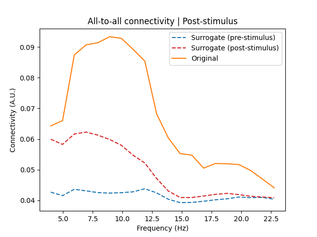
Plotting the post-stimulus connectivity against the estimates from both sets of surrogate data, we see that the surrogate data from the inappropriate method (make_surrogate_resting_data()) greatly overestimates the baseline connectivity in the alpha band.

Although the alpha connectivity was still far above the baseline from the evoked surrogates, this will not always be the case. You can see how this risks false negative assessments that connectivity is not significantly different from baseline. Surrogate connectivity estimates from evoked data should therefore always be generated using the make_surrogate_evoked_data() function.

# Plot post-stimulus actual vs. surrogate connectivity
fig, ax = plt.subplots(1, 1)
ax.plot(
    freqs,
    poststim_surrogate_con.mean(axis=0),
    linestyle="--",
    label="Surrogate\n(make_surrogate_evoked_data)",
)
ax.plot(
    freqs,
    bad_surrogate_con.mean(axis=0),
    color="C3",
    linestyle="--",
    label="Surrogate\n(make_surrogate_resting_data)",
)
ax.plot(freqs, poststim_con, color="C1", label="Original")
ax.set_xlabel("Frequency (Hz)")
ax.set_ylabel("Connectivity (A.U.)")
ax.set_title("All-to-all connectivity | Post-stimulus")
ax.legend()

<matplotlib.legend.Legend object at 0x763d939ee7b0>

Assessing connectivity on a group-level

While our focus here has been on assessing the significance of connectivity on a single-recording-level, we may also want to determine whether group-level connectivity estimates are significantly different from baseline. For this, we can generate surrogates and estimate connectivity alongside the original signals for each piece of data.

There are multiple ways to assess the statistical significance. For example, we can compute p-values for each piece of data using the approach above and combine them for the nested data (e.g., across recordings, subjects, etc…) using Stouffer’s method [4].

Alternatively, we could take the average of the surrogate connectivity estimates across all shuffles for each piece of data and compare them to the original connectivity estimates in a paired test. The scipy.stats and mne.stats modules have many such tools for testing this, e.g., scipy.stats.ttest_1samp(), mne.stats.permutation_t_test(), etc…

Altogether, surrogate connectivity estimates are a powerful tool for assessing the significance of connectivity estimates, both on a single recording- and group-level.

References

[1]

Martin Vinck, Marijn van Wingerden, Thilo Womelsdorf, Pascal Fries, and Cyriel M.A. Pennartz. The pairwise phase consistency: a bias-free measure of rhythmic neuronal synchronization. NeuroImage, 51(1):112–122, 2010. doi:10.1016/j.neuroimage.2010.01.073.

[2] (1,2)

Franziska Pellegrini, Arnaud Delorme, Vadim Nikulin, and Stefan Haufe. Identifying good practices for detecting inter-regional linear functional connectivity from EEG. NeuroImage, 277:120218, 2023. doi:10.1016/j.neuroimage.2023.120218.

[3]

Juhan Aru, Jaan Aru, Viola Priesemann, Michael Wibral, Luiz Lana, Gordon Pipa, Wolf Singer, and Raul Vicente. Untangling cross-frequency coupling in neuroscience. Current Opinion in Neurobiology, 31:51–61, 2015. doi:10.1016/j.conb.2014.08.002.

[4]

Irene Dowding and Stefan Haufe. Powerful statistical inference for nested data using sufficient summary statistics. Frontiers in Human Neuroscience, 12:103, 2018. doi:10.3389/fnhum.2018.00103.