Comparison of coherency-based methods

This example demonstrates the distinct forms of information captured by coherency-based connectivity methods, and highlights the scenarios in which these different methods should be applied.

# Authors: Thomas S. Binns <t.s.binns@outlook.com>
#          Mohammad Orabe <orabe.mhd@gmail.com>
# License: BSD (3-clause)

import numpy as np
from matplotlib import pyplot as plt

from mne_connectivity import (
    make_signals_in_freq_bands,
    seed_target_indices,
    spectral_connectivity_epochs,
)

An introduction to coherency-based connectivity methods

MNE-Connectivity supports several methods based on coherency. These are:

• coherency (Cohy)

• coherence (Coh; absolute coherency)

• imaginary part of coherency (ImCoh)

• canonical coherency (CaCoh)

• maximised imaginary part of coherency (MIC)

• multivariate interaction measure (MIM)

All of these methods centre on Cohy, a complex-valued estimate of the correlation between signals in the frequency domain. It is an undirected measure of connectivity, being invariant to the direction of information flow between signals.

The common approach for handling these complex-valued coherency scores is to either take their absolute values (Coh) or their imaginary values (ImCoh [1]).

In addition to these traditional bivariate connectivity measures (i.e. between two signals), advanced multivariate measures (i.e. between groups of signals) have also been developed based on Cohy (CaCoh [2]; can take the absolute value for a multivariate form of Coh; see Compute multivariate coherency/coherence) or ImCoh (MIC & MIM [3]; see Compute multivariate measures of the imaginary part of coherency).

Despite their similarities, there are distinct scenarios in which these different methods are most appropriate, as we will show in this example.

Zero and non-zero time-lag interactions

The key difference between Cohy/Coh and ImCoh is how information about zero time-lag interactions is captured.

We generally assume that communication within the brain involves some delay in the flow of information (i.e. a non-zero time-lag). This reflects the time taken for: the propagation of action potentials along axons; the release of neurotransmitters from presynaptic terminals and binding to receptors on postsynaptic terminals; etc…

In contrast, interactions with no delay (i.e. a zero time-lag) are often considered to reflect non-physiological activity, such as volume conduction - the propagation of electrical activity through the brain’s conductive tissue from a single source to multiple electrodes simultaneously [1]. Such interactions therefore do not reflect genuine, physiological communication between brain regions. Naturally, having a method that can discard spurious zero time-lag connectivity estimates is very desirable.

Note: Not all zero time-lag interactions are necessarily non-physiological [4].

To demonstrate the differences in how Cohy/Coh and ImCoh handle zero time-lag interactions, we simulate two sets of data with:

1. A non-zero time-lag interaction at 10-12 Hz.

2. A zero time-lag interaction at 23-25 Hz.

# Generate simulated data
data_delay = make_signals_in_freq_bands(
    n_seeds=3,
    n_targets=3,
    freq_band=(10, 12),  # 10-12 Hz interaction
    connection_delay=2,  # samples; non-zero time-lag
    rng_seed=42,
)

data_no_delay = make_signals_in_freq_bands(
    n_seeds=3,
    n_targets=3,
    freq_band=(23, 25),  # 23-25 Hz interaction
    connection_delay=0,  # samples; zero time-lag
    rng_seed=44,
)

# Combine data into a single object
data = data_delay.add_channels([data_no_delay])

Setting up band-pass filter from 10 - 12 Hz

FIR filter parameters
---------------------
Designing a one-pass, zero-phase, non-causal bandpass filter:
- Windowed frequency-domain design (firwin2) method
- Hamming window
- Lower passband edge: 10.00
- Lower transition bandwidth: 1.00 Hz (-6 dB cutoff frequency: 9.50 Hz)
- Upper passband edge: 12.00 Hz
- Upper transition bandwidth: 1.00 Hz (-6 dB cutoff frequency: 12.50 Hz)
- Filter length: 661 samples (6.610 s)

Not setting metadata
10 matching events found
No baseline correction applied
0 projection items activated
Setting up band-pass filter from 23 - 25 Hz

FIR filter parameters
---------------------
Designing a one-pass, zero-phase, non-causal bandpass filter:
- Windowed frequency-domain design (firwin2) method
- Hamming window
- Lower passband edge: 23.00
- Lower transition bandwidth: 1.00 Hz (-6 dB cutoff frequency: 22.50 Hz)
- Upper passband edge: 25.00 Hz
- Upper transition bandwidth: 1.00 Hz (-6 dB cutoff frequency: 25.50 Hz)
- Filter length: 661 samples (6.610 s)

Not setting metadata
10 matching events found
No baseline correction applied
0 projection items activated

We compute the connectivity of these simulated signals using CaCoh (a multivariate form of Cohy/Coh) and MIC (a multivariate form of ImCoh).

# Generate connectivity indices
seeds = [0, 1, 2, 6, 7, 8]
targets = [3, 4, 5, 9, 10, 11]
bivar_indices = seed_target_indices(seeds, targets)
multivar_indices = ([seeds], [targets])

# Compute CaCoh & MIC
(cacoh, mic) = spectral_connectivity_epochs(
    data, method=["cacoh", "mic"], indices=multivar_indices, sfreq=100, fmin=3, fmax=35
)

/home/circleci/project/mne_connectivity/spectral/epochs.py:995: RuntimeWarning: There were no Annotations stored in <EpochsArray |  10 events (all good), 0 – 1.99 s, baseline off, ~204 kB, data loaded,
 '1': 10>, so metadata was not modified.
  data.add_annotations_to_metadata(overwrite=True)
Connectivity computation...
    computing connectivity for 1 connections
    using t=0.000s..1.990s for estimation (200 points)
    frequencies: 3.0Hz..35.0Hz (65 points)
Estimated data ranks:
    connection 1 - seeds (6); targets (6)
    Using multitaper spectrum estimation with 7 DPSS windows
    the following metrics will be computed: CaCoh, MIC
    computing cross-spectral density for epoch 1
    computing cross-spectral density for epoch 2
    computing cross-spectral density for epoch 3
    computing cross-spectral density for epoch 4
    computing cross-spectral density for epoch 5
    computing cross-spectral density for epoch 6
    computing cross-spectral density for epoch 7
    computing cross-spectral density for epoch 8
    computing cross-spectral density for epoch 9
    computing cross-spectral density for epoch 10
Computing CaCoh for connection 1 of 1

  0%|          | frequency blocks : 0/65 [00:00<?,       ?it/s]
  6%|▌         | frequency blocks : 4/65 [00:00<00:00,  202.26it/s]
 12%|█▏        | frequency blocks : 8/65 [00:00<00:00,  203.79it/s]
 18%|█▊        | frequency blocks : 12/65 [00:00<00:00,  214.89it/s]
 25%|██▍       | frequency blocks : 16/65 [00:00<00:00,  137.01it/s]
 31%|███       | frequency blocks : 20/65 [00:00<00:00,  150.98it/s]
 37%|███▋      | frequency blocks : 24/65 [00:00<00:00,  161.87it/s]
 42%|████▏     | frequency blocks : 27/65 [00:00<00:00,  122.29it/s]
 46%|████▌     | frequency blocks : 30/65 [00:00<00:00,  127.36it/s]
 52%|█████▏    | frequency blocks : 34/65 [00:00<00:00,  136.31it/s]
 58%|█████▊    | frequency blocks : 38/65 [00:00<00:00,  144.09it/s]
 60%|██████    | frequency blocks : 39/65 [00:00<00:00,  120.00it/s]
 66%|██████▌   | frequency blocks : 43/65 [00:00<00:00,  127.61it/s]
 72%|███████▏  | frequency blocks : 47/65 [00:00<00:00,  134.81it/s]
 78%|███████▊  | frequency blocks : 51/65 [00:00<00:00,  139.92it/s]
 80%|████████  | frequency blocks : 52/65 [00:00<00:00,  120.36it/s]
 86%|████████▌ | frequency blocks : 56/65 [00:00<00:00,  126.72it/s]
 92%|█████████▏| frequency blocks : 60/65 [00:00<00:00,  131.59it/s]
 98%|█████████▊| frequency blocks : 64/65 [00:00<00:00,  119.80it/s]
100%|██████████| frequency blocks : 65/65 [00:00<00:00,  125.29it/s]
Computing MIC for connection 1 of 1

  0%|          | frequency blocks : 0/65 [00:00<?,       ?it/s]
  5%|▍         | frequency blocks : 3/65 [00:00<00:01,   52.03it/s]
 11%|█         | frequency blocks : 7/65 [00:00<00:00,   95.79it/s]
 17%|█▋        | frequency blocks : 11/65 [00:00<00:00,  124.10it/s]
 23%|██▎       | frequency blocks : 15/65 [00:00<00:00,  143.59it/s]
 25%|██▍       | frequency blocks : 16/65 [00:00<00:00,  101.18it/s]
 31%|███       | frequency blocks : 20/65 [00:00<00:00,  116.11it/s]
 37%|███▋      | frequency blocks : 24/65 [00:00<00:00,  128.95it/s]
 43%|████▎     | frequency blocks : 28/65 [00:00<00:00,  139.72it/s]
 45%|████▍     | frequency blocks : 29/65 [00:00<00:00,  111.82it/s]
 51%|█████     | frequency blocks : 33/65 [00:00<00:00,  121.27it/s]
 57%|█████▋    | frequency blocks : 37/65 [00:00<00:00,  129.99it/s]
 63%|██████▎   | frequency blocks : 41/65 [00:00<00:00,  138.35it/s]
 66%|██████▌   | frequency blocks : 43/65 [00:00<00:00,  118.57it/s]
 72%|███████▏  | frequency blocks : 47/65 [00:00<00:00,  125.89it/s]
 78%|███████▊  | frequency blocks : 51/65 [00:00<00:00,  132.55it/s]
 85%|████████▍ | frequency blocks : 55/65 [00:00<00:00,  138.77it/s]
 86%|████████▌ | frequency blocks : 56/65 [00:00<00:00,  120.25it/s]
 92%|█████████▏| frequency blocks : 60/65 [00:00<00:00,  126.26it/s]
 98%|█████████▊| frequency blocks : 64/65 [00:00<00:00,  132.14it/s]
100%|██████████| frequency blocks : 65/65 [00:00<00:00,  130.17it/s]
[Connectivity computation done]

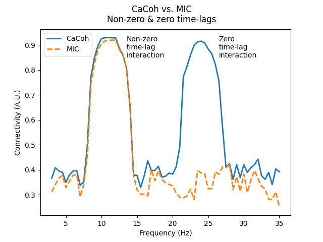
As you can see, both CaCoh and MIC capture the non-zero time-lag interaction at 10-12 Hz, however only CaCoh captures the zero time-lag interaction at 23-25 Hz.

# Plot CaCoh & MIC
fig, axis = plt.subplots(1, 1)
axis.plot(cacoh.freqs, np.abs(cacoh.get_data()[0]), linewidth=2, label="CaCoh")
axis.plot(
    mic.freqs, np.abs(mic.get_data()[0]), linewidth=2, label="MIC", linestyle="--"
)
axis.set_xlabel("Frequency (Hz)")
axis.set_ylabel("Connectivity (A.U.)")
axis.annotate("Non-zero\ntime-lag\ninteraction", xy=(13.5, 0.85))
axis.annotate("Zero\ntime-lag\ninteraction", xy=(26.5, 0.85))
axis.legend(loc="upper left")
fig.suptitle("CaCoh vs. MIC\nNon-zero & zero time-lags")

Text(0.5, 0.98, 'CaCoh vs. MIC\nNon-zero & zero time-lags')

def plot_connectivity_circle():
    """Plot a circle with radius 1, real and imag. axes, and angles marked."""
    fig, axis = plt.subplots(1, 1)
    t = np.linspace(0, 2 * np.pi, 100)
    axis.plot(np.cos(t), np.sin(t), color="k", linewidth=0.1)
    axis.plot([-1, 1], [0, 0], color="k", linestyle="--")
    axis.plot([0, 0], [-1, 1], color="k", linestyle="--")
    axis.axis("off")

    fontdict = {"fontsize": 10}
    qpi = np.pi / 4
    axis.text(1, 0, " 0°", ha="left", va="center", fontdict=fontdict)
    axis.text(np.pi / 4, np.pi / 4, "45°", ha="center", va="center", fontdict=fontdict)
    axis.text(0, 1, "90°", ha="center", va="bottom", fontdict=fontdict)
    axis.text(-qpi, qpi, "135°", ha="center", va="center", fontdict=fontdict)
    axis.text(-1, 0, "180°", ha="right", va="center", fontdict=fontdict)
    axis.text(-qpi, -qpi, "-135°", ha="center", va="center", fontdict=fontdict)
    axis.text(0, -1, "-90°", ha="center", va="top", fontdict=fontdict)
    axis.text(qpi, -qpi, "-45°", ha="center", va="center", fontdict=fontdict)

    fontdict = {"fontsize": 12}
    axis.text(1.15, 0, " Real", ha="left", va="center", fontdict=fontdict)
    axis.text(0, 1.15, "Imaginary", ha="center", va="bottom", fontdict=fontdict)
    axis.text(0, 0, "0 ", ha="right", va="top", fontdict=fontdict)
    axis.text(-1, 0, "-1", ha="left", va="top", fontdict=fontdict)
    axis.text(1, 0, "+1", ha="right", va="top", fontdict=fontdict)
    axis.text(0, -1, "-1 ", ha="right", va="bottom", fontdict=fontdict)
    axis.text(0, 1, "+1 ", ha="right", va="top", fontdict=fontdict)

    axis.set_aspect("equal")

    return fig, axis

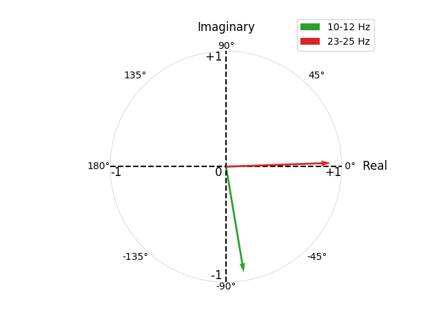
The different interactions (not) captured by CaCoh and MIC can be understood by visualising the complex values of the interactions.

# Get complex connectivity values at frequency bands
freqs = cacoh.freqs
cacoh_10_12 = np.mean(cacoh.get_data()[0, freqs.index(10) : freqs.index(12) + 1])
cacoh_23_25 = np.mean(cacoh.get_data()[0, freqs.index(23) : freqs.index(25) + 1])

# Plot complex connectivity values
fig, axis = plot_connectivity_circle()
axis.quiver(
    0,
    0,
    np.real(cacoh_10_12),
    np.imag(cacoh_10_12),
    units="xy",
    scale=1,
    linewidth=2,
    color="C2",
    label="10-12 Hz",
)
axis.quiver(
    0,
    0,
    np.real(cacoh_23_25),
    np.imag(cacoh_23_25),
    units="xy",
    scale=1,
    linewidth=2,
    color="C3",
    label="23-25 Hz",
    zorder=99,
)
axis.legend(loc="upper right", bbox_to_anchor=[1.1, 1.1])

<matplotlib.legend.Legend object at 0x7fb912c93430>

Above, we plot the complex-valued CaCoh scores for the 10-12 Hz and 23-25 Hz interactions as vectors with origin \((0, 0)\) bound within a circle of radius 1 (reflecting the fact that coherency scores span the set of complex values in the range \([-1, 1]\)).

The circumference of the circle spans the range \((-\pi, \pi]\). The real axis corresponds to vectors with angles of 0° (\(0\pi\); positive values) or 180° (\(\pi\); negative values). The imaginary axis corresponds to vectors with angles of 90° (\(\frac{1}{2}\pi\); positive values) or -90° (\(-\frac{1}{2}\pi\); negative values).

Zero time-lag interactions have angles of 0° and 180° (i.e. no phase difference), corresponding to a non-zero real component, but a zero-valued imaginary component. We see this nicely for the 23-25 Hz interaction, which has an angle of ~0°. Taking the absolute CaCoh value shows us the magnitude of this interaction to be ~0.9. However, first projecting this information to the imaginary axis gives us a magnitude of ~0.

In contrast, non-zero time-lag interactions do not lie on the real axis (i.e. a phase difference), corresponding to non-zero real and imaginary components. We see this nicely for the 10-12 Hz interaction, which has an angle of ~-75°. Taking the absolute CaCoh value shows us the magnitude of this interaction to be ~0.9, which is also seen when first projecting this information to the imaginary axis.

This distinction is why connectivity methods utilising information from both real and imaginary components (Cohy, Coh, CaCoh) capture both zero and non-zero time-lag interactions, whereas methods using only the imaginary component (ImCoh, MIC, MIM) capture only non-zero time-lag interactions.

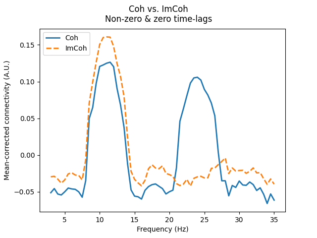
The ability to capture these different interactions is not a feature specific to multivariate connectivity methods, as shown below for the bivariate methods Coh and ImCoh.

# Compute Coh & ImCoh
(coh, imcoh) = spectral_connectivity_epochs(
    data, method=["coh", "imcoh"], indices=bivar_indices, sfreq=100, fmin=3, fmax=35
)

coh_mean = np.mean(coh.get_data(), axis=0)
imcoh_mean = np.mean(np.abs(imcoh.get_data()), axis=0)

coh_mean_subbed = coh_mean - np.mean(coh_mean)
imcoh_mean_subbed = imcoh_mean - np.mean(imcoh_mean)

# Plot Coh & ImCoh
fig, axis = plt.subplots(1, 1)
axis.plot(coh.freqs, coh_mean_subbed, linewidth=2, label="Coh")
axis.plot(imcoh.freqs, imcoh_mean_subbed, linewidth=2, label="ImCoh", linestyle="--")
axis.set_xlabel("Frequency (Hz)")
axis.set_ylabel("Mean-corrected connectivity (A.U.)")
axis.annotate("Non-zero\ntime-lag\ninteraction", xy=(13, 0.25))
axis.annotate("Zero\ntime-lag\ninteraction", xy=(25, 0.25))
axis.legend(loc="upper left")
fig.suptitle("Coh vs. ImCoh\nNon-zero & zero time-lags")

/home/circleci/project/mne_connectivity/spectral/epochs.py:995: RuntimeWarning: There were no Annotations stored in <EpochsArray |  10 events (all good), 0 – 1.99 s, baseline off, ~204 kB, data loaded,
 '1': 10>, so metadata was not modified.
  data.add_annotations_to_metadata(overwrite=True)
Connectivity computation...
    computing connectivity for 36 connections
    using t=0.000s..1.990s for estimation (200 points)
    frequencies: 3.0Hz..35.0Hz (65 points)
    Using multitaper spectrum estimation with 7 DPSS windows
    the following metrics will be computed: Coherence, Imaginary Coherence
    computing cross-spectral density for epoch 1
    computing cross-spectral density for epoch 2
    computing cross-spectral density for epoch 3
    computing cross-spectral density for epoch 4
    computing cross-spectral density for epoch 5
    computing cross-spectral density for epoch 6
    computing cross-spectral density for epoch 7
    computing cross-spectral density for epoch 8
    computing cross-spectral density for epoch 9
    computing cross-spectral density for epoch 10
[Connectivity computation done]

Text(0.5, 0.98, 'Coh vs. ImCoh\nNon-zero & zero time-lags')

When different coherency-based methods are most appropriate

With this information, we can define situations under which these different approaches are most appropriate.

In situations where non-physiological zero time-lag interactions are assumed, methods based on only the imaginary part of coherency (ImCoh, MIC, MIM) should be used. Examples of situations include:

• Connectivity between channels of a single modality.

• Connectivity between channels of different modalities where the same reference is used.

Note that this applies not only to sensor-space signals, but also to source-space signals where remnants of these non-physiological interactions may remain even after source reconstruction.

In situations where non-physiological zero time-lag interactions are not assumed, methods based on real and imaginary parts of coherency (Cohy, Coh, CaCoh) should be used. An example includes:

• Connectivity between channels of different modalities where different references are used.

Equally, when there are no non-physiological zero time-lag interactions, one should not used methods based on only the imaginary part of coherency. There are two key reasons:

1. Discarding physiological zero time-lag interactions

First, not all zero time-lag interactions are non-physiological [4]. Accordingly, methods based on only the imaginary part of coherency may lead to information about genuine connectivity being lost.

In situations where non-physiological zero time-lag interactions are present, the potential loss of physiological information is generally acceptable to avoid spurious connectivity estimates. However, unnecessarily discarding this information can of course be detrimental.

2. Biasing interactions based on the angle of interaction

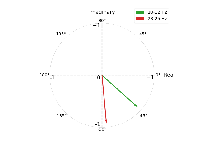
Depending on their angles, two non-zero time-lag interactions may have the same magnitude in the complex plane, but different magnitudes when projected to the imaginary axis.

This is demonstrated below, where we simulate 2 interactions with non-zero time-lags at 10-12 Hz and 23-25 Hz. Computing the connectivity, we see how both interactions have a similar magnitude (~0.9), but different angles (~-45° for 10-12 Hz; ~-90° for 23-25 Hz).

# Generate simulated data
data_10_12 = make_signals_in_freq_bands(
    n_seeds=3,
    n_targets=3,
    freq_band=(10, 12),  # 10-12 Hz interaction
    connection_delay=1,  # samples
    rng_seed=40,
)

data_23_25 = make_signals_in_freq_bands(
    n_seeds=3,
    n_targets=3,
    freq_band=(23, 25),  # 23-25 Hz interaction
    connection_delay=1,  # samples
    rng_seed=42,
)

# Combine data into a single array
data = data_10_12.add_channels([data_23_25])

# Compute CaCoh & MIC
(cacoh, mic) = spectral_connectivity_epochs(
    data, method=["cacoh", "mic"], indices=multivar_indices, sfreq=100, fmin=3, fmax=35
)

# Get complex connectivity values at frequency bands
freqs = cacoh.freqs
cacoh_10_12 = np.mean(cacoh.get_data()[0, freqs.index(10) : freqs.index(12) + 1])
cacoh_23_25 = np.mean(cacoh.get_data()[0, freqs.index(23) : freqs.index(25) + 1])

# Plot complex connectivity values
fig, axis = plot_connectivity_circle()
axis.quiver(
    0,
    0,
    np.real(cacoh_10_12),
    np.imag(cacoh_10_12),
    units="xy",
    scale=1,
    linewidth=2,
    color="C2",
    label="10-12 Hz",
)
axis.quiver(
    0,
    0,
    np.real(cacoh_23_25),
    np.imag(cacoh_23_25),
    units="xy",
    scale=1,
    linewidth=2,
    color="C3",
    label="23-25 Hz",
    zorder=99,
)
axis.legend(loc="upper right", bbox_to_anchor=[1.1, 1.1])

Setting up band-pass filter from 10 - 12 Hz

FIR filter parameters
---------------------
Designing a one-pass, zero-phase, non-causal bandpass filter:
- Windowed frequency-domain design (firwin2) method
- Hamming window
- Lower passband edge: 10.00
- Lower transition bandwidth: 1.00 Hz (-6 dB cutoff frequency: 9.50 Hz)
- Upper passband edge: 12.00 Hz
- Upper transition bandwidth: 1.00 Hz (-6 dB cutoff frequency: 12.50 Hz)
- Filter length: 661 samples (6.610 s)

Not setting metadata
10 matching events found
No baseline correction applied
0 projection items activated
Setting up band-pass filter from 23 - 25 Hz

FIR filter parameters
---------------------
Designing a one-pass, zero-phase, non-causal bandpass filter:
- Windowed frequency-domain design (firwin2) method
- Hamming window
- Lower passband edge: 23.00
- Lower transition bandwidth: 1.00 Hz (-6 dB cutoff frequency: 22.50 Hz)
- Upper passband edge: 25.00 Hz
- Upper transition bandwidth: 1.00 Hz (-6 dB cutoff frequency: 25.50 Hz)
- Filter length: 661 samples (6.610 s)

Not setting metadata
10 matching events found
No baseline correction applied
0 projection items activated
/home/circleci/project/mne_connectivity/spectral/epochs.py:995: RuntimeWarning: There were no Annotations stored in <EpochsArray |  10 events (all good), 0 – 1.99 s, baseline off, ~204 kB, data loaded,
 '1': 10>, so metadata was not modified.
  data.add_annotations_to_metadata(overwrite=True)
Connectivity computation...
    computing connectivity for 1 connections
    using t=0.000s..1.990s for estimation (200 points)
    frequencies: 3.0Hz..35.0Hz (65 points)
Estimated data ranks:
    connection 1 - seeds (6); targets (6)
    Using multitaper spectrum estimation with 7 DPSS windows
    the following metrics will be computed: CaCoh, MIC
    computing cross-spectral density for epoch 1
    computing cross-spectral density for epoch 2
    computing cross-spectral density for epoch 3
    computing cross-spectral density for epoch 4
    computing cross-spectral density for epoch 5
    computing cross-spectral density for epoch 6
    computing cross-spectral density for epoch 7
    computing cross-spectral density for epoch 8
    computing cross-spectral density for epoch 9
    computing cross-spectral density for epoch 10
Computing CaCoh for connection 1 of 1

  0%|          | frequency blocks : 0/65 [00:00<?,       ?it/s]
  5%|▍         | frequency blocks : 3/65 [00:00<00:00,  176.97it/s]
  9%|▉         | frequency blocks : 6/65 [00:00<00:00,  173.26it/s]
 15%|█▌        | frequency blocks : 10/65 [00:00<00:00,  174.99it/s]
 22%|██▏       | frequency blocks : 14/65 [00:00<00:00,  189.33it/s]
 28%|██▊       | frequency blocks : 18/65 [00:00<00:00,  198.78it/s]
 34%|███▍      | frequency blocks : 22/65 [00:00<00:00,  206.73it/s]
 35%|███▌      | frequency blocks : 23/65 [00:00<00:00,  140.84it/s]
 42%|████▏     | frequency blocks : 27/65 [00:00<00:00,  148.71it/s]
 48%|████▊     | frequency blocks : 31/65 [00:00<00:00,  158.30it/s]
 54%|█████▍    | frequency blocks : 35/65 [00:00<00:00,  166.56it/s]
 55%|█████▌    | frequency blocks : 36/65 [00:00<00:00,  132.03it/s]
 62%|██████▏   | frequency blocks : 40/65 [00:00<00:00,  140.16it/s]
 68%|██████▊   | frequency blocks : 44/65 [00:00<00:00,  147.81it/s]
 74%|███████▍  | frequency blocks : 48/65 [00:00<00:00,  154.75it/s]
 75%|███████▌  | frequency blocks : 49/65 [00:00<00:00,  130.09it/s]
 82%|████████▏ | frequency blocks : 53/65 [00:00<00:00,  136.74it/s]
 88%|████████▊ | frequency blocks : 57/65 [00:00<00:00,  143.09it/s]
 94%|█████████▍| frequency blocks : 61/65 [00:00<00:00,  148.85it/s]
 95%|█████████▌| frequency blocks : 62/65 [00:00<00:00,  128.67it/s]
100%|██████████| frequency blocks : 65/65 [00:00<00:00,  138.31it/s]
Computing MIC for connection 1 of 1

  0%|          | frequency blocks : 0/65 [00:00<?,       ?it/s]
  5%|▍         | frequency blocks : 3/65 [00:00<00:01,   52.20it/s]
 11%|█         | frequency blocks : 7/65 [00:00<00:00,   95.34it/s]
 17%|█▋        | frequency blocks : 11/65 [00:00<00:00,  123.56it/s]
 23%|██▎       | frequency blocks : 15/65 [00:00<00:00,  143.48it/s]
 25%|██▍       | frequency blocks : 16/65 [00:00<00:00,  100.63it/s]
 31%|███       | frequency blocks : 20/65 [00:00<00:00,  115.72it/s]
 37%|███▋      | frequency blocks : 24/65 [00:00<00:00,  127.86it/s]
 43%|████▎     | frequency blocks : 28/65 [00:00<00:00,  138.73it/s]
 45%|████▍     | frequency blocks : 29/65 [00:00<00:00,  111.16it/s]
 51%|█████     | frequency blocks : 33/65 [00:00<00:00,  121.19it/s]
 57%|█████▋    | frequency blocks : 37/65 [00:00<00:00,  130.30it/s]
 63%|██████▎   | frequency blocks : 41/65 [00:00<00:00,  138.25it/s]
 65%|██████▍   | frequency blocks : 42/65 [00:00<00:00,  116.35it/s]
 71%|███████   | frequency blocks : 46/65 [00:00<00:00,  124.14it/s]
 77%|███████▋  | frequency blocks : 50/65 [00:00<00:00,  130.94it/s]
 83%|████████▎ | frequency blocks : 54/65 [00:00<00:00,  137.42it/s]
 85%|████████▍ | frequency blocks : 55/65 [00:00<00:00,  118.79it/s]
 91%|█████████ | frequency blocks : 59/65 [00:00<00:00,  125.25it/s]
 97%|█████████▋| frequency blocks : 63/65 [00:00<00:00,  131.35it/s]
100%|██████████| frequency blocks : 65/65 [00:00<00:00,  130.22it/s]
[Connectivity computation done]

<matplotlib.legend.Legend object at 0x7fb912f99810>

Plotting the connectivity values for CaCoh and MIC, we see how the 10-12 Hz and 23-25 Hz interactions have a similar magnitude for CaCoh, whereas the MIC scores for the 10-12 Hz interaction are lower than for the 23-25 Hz interaction.

This difference reflects the fact that as the angle of interaction deviates from \(\pm\) 90°, less information will be represented in the imaginary part of coherency. Accordingly, considering only the imaginary part of coherency can bias connectivity estimates based on the angle of interaction.

# Plot CaCoh & MIC
fig, axis = plt.subplots(1, 1)
axis.plot(cacoh.freqs, np.abs(cacoh.get_data()[0]), linewidth=2, label="CaCoh")
axis.plot(
    mic.freqs, np.abs(mic.get_data()[0]), linewidth=2, label="MIC", linestyle="--"
)
axis.set_xlabel("Frequency (Hz)")
axis.set_ylabel("Connectivity (A.U.)")
axis.annotate("$\pm$45°\ninteraction", xy=(12.5, 0.9))
axis.annotate("$\pm$90°\ninteraction", xy=(26.5, 0.9))
axis.legend(loc="upper left")
fig.suptitle("CaCoh vs. MIC\n$\pm$45° & $\pm$90° interactions")

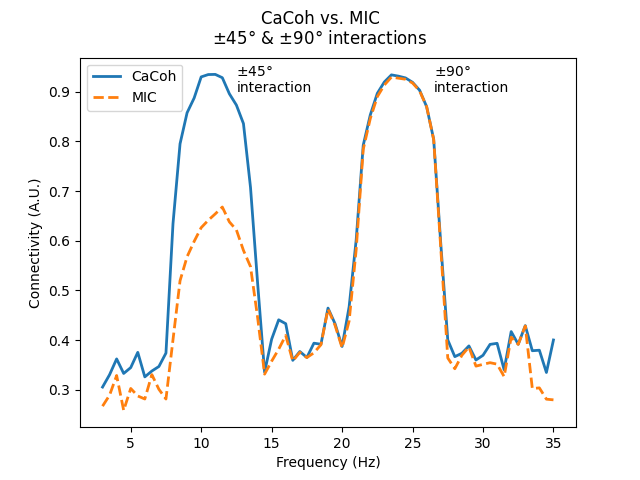
Text(0.5, 0.98, 'CaCoh vs. MIC\n$\\pm$45° & $\\pm$90° interactions')

In situations where non-physiological zero time-lag interactions are present, this phase angle-dependent bias is generally acceptable to avoid spurious connectivity estimates. However in situations where non-physiological zero time-lag interactions are not present, such a bias is clearly problematic.

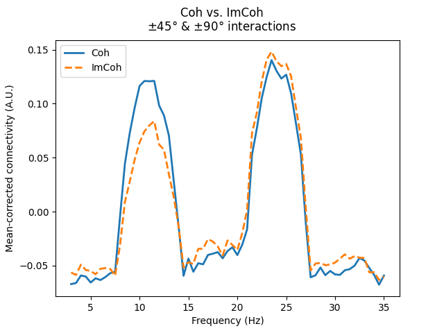
Again, these considerations are not specific to multivariate methods, as shown below with Coh and ImCoh.

# Compute Coh & ImCoh
(coh, imcoh) = spectral_connectivity_epochs(
    data, method=["coh", "imcoh"], indices=bivar_indices, sfreq=100, fmin=3, fmax=35
)

coh_mean = np.mean(coh.get_data(), axis=0)
imcoh_mean = np.mean(np.abs(imcoh.get_data()), axis=0)

coh_mean_subbed = coh_mean - np.mean(coh_mean)
imcoh_mean_subbed = imcoh_mean - np.mean(imcoh_mean)

# Plot Coh & ImCoh
fig, axis = plt.subplots(1, 1)
axis.plot(coh.freqs, coh_mean_subbed, linewidth=2, label="Coh")
axis.plot(imcoh.freqs, imcoh_mean_subbed, linewidth=2, label="ImCoh", linestyle="--")
axis.set_xlabel("Frequency (Hz)")
axis.set_ylabel("Mean-corrected connectivity (A.U.)")
axis.annotate("$\pm$45°\ninteraction", xy=(13, 0.25))
axis.annotate("$\pm$90°\ninteraction", xy=(26.5, 0.25))
axis.legend(loc="upper left")
fig.suptitle("Coh vs. ImCoh\n$\pm$45° & $\pm$90° interactions")

/home/circleci/project/mne_connectivity/spectral/epochs.py:995: RuntimeWarning: There were no Annotations stored in <EpochsArray |  10 events (all good), 0 – 1.99 s, baseline off, ~204 kB, data loaded,
 '1': 10>, so metadata was not modified.
  data.add_annotations_to_metadata(overwrite=True)
Connectivity computation...
    computing connectivity for 36 connections
    using t=0.000s..1.990s for estimation (200 points)
    frequencies: 3.0Hz..35.0Hz (65 points)
    Using multitaper spectrum estimation with 7 DPSS windows
    the following metrics will be computed: Coherence, Imaginary Coherence
    computing cross-spectral density for epoch 1
    computing cross-spectral density for epoch 2
    computing cross-spectral density for epoch 3
    computing cross-spectral density for epoch 4
    computing cross-spectral density for epoch 5
    computing cross-spectral density for epoch 6
    computing cross-spectral density for epoch 7
    computing cross-spectral density for epoch 8
    computing cross-spectral density for epoch 9
    computing cross-spectral density for epoch 10
[Connectivity computation done]

Text(0.5, 0.98, 'Coh vs. ImCoh\n$\\pm$45° & $\\pm$90° interactions')

Bivariate vs. multivariate coherency methods

As we have seen, coherency-based methods can be bivariate (Cohy, Coh, ImCoh) and multivariate (CaCoh, MIC, MIM). Whilst both forms capture the same information, there are several benefits to using multivariate methods when investigating connectivity between many signals.

The multivariate methods can be used to capture the most relevant interactions between two groups of signals, representing this information in the component, rather than signal space.

The dimensionality reduction associated with these methods offers: a much easier interpretation of the results; a higher signal-to-noise ratio compared to e.g. averaging bivariate connectivity estimates across multiple pairs of signals; and even reduced bias in what information is captured [3].

Furthermore, despite the dimensionality reduction of multivariate methods it is still possible to investigate the topographies of connectivity, with spatial patterns of connectivity being returned alongside the connectivity values themselves [5].

More information about the multivariate coherency-based methods can be found in the following examples:

• CaCoh - Compute multivariate coherency/coherence

• MIC & MIM - Compute multivariate measures of the imaginary part of coherency

Alternative approaches to computing connectivity

Coherency-based methods are only some of the many approaches available in MNE-Connectivity for studying interactions between signals. Other non-directed measures include those based on the phase-lag index [6][7] (see also Comparing PLI, wPLI, and dPLI) and phase locking value [8][9].

Furthermore, directed measures of connectivity which determine the direction of information flow are also available, including a variant of the phase-lag index [10] (see also Comparing PLI, wPLI, and dPLI), the phase slope index [11] (see also mne_connectivity.phase_slope_index()), and Granger causality [12][13] (see also Compute directionality of connectivity with multivariate Granger causality).

Conclusion

Altogether, there are clear scenarious in which different coherency-based methods are appropriate.

Methods based on the imaginary part of coherency alone (ImCoh, MIC, MIM) should be used when non-physiological zero time-lag interactions are present.

In contrast, methods based on the real and imaginary parts of coherency (Cohy, Coh, CaCoh) should be used when non-physiological zero time-lag interactions are absent.

References

[1] (1,2)

Guido Nolte, Ou Bai, Lewis Wheaton, Zoltan Mari, Sherry Vorbach, and Mark Hallett. Identifying true brain interaction from EEG data using the imaginary part of coherency. Clinical Neurophysiology, 115(10):2292–2307, 2004. doi:10.1016/j.clinph.2004.04.029.

[2]

Carmen Vidaurre, Guido Nolte, Ingmar E.J. de Vries, M. Gómez, Tjeerd W. Boonstra, K.-R. Müller, Arno Villringer, and Vadim V. Nikulin. Canonical maximization of coherence: a novel tool for investigation of neuronal interactions between two datasets. NeuroImage, 201:116009, 2019. doi:10.1016/j.neuroimage.2019.116009.

[3] (1,2)

Arne Ewald, Laura Marzetti, Filippo Zappasodi, Frank C. Meinecke, and Guido Nolte. Estimating true brain connectivity from EEG/MEG data invariant to linear and static transformations in sensor space. NeuroImage, 60(1):476–488, 2012. doi:10.1016/j.neuroimage.2011.11.084.

[4] (1,2)

Atthaphon Viriyopase, Ingo Bojak, Magteld Zeitler, and Stan Gielen. When long-range zero-lag synchronization is feasible in cortical networks. Frontiers in Computational Neuroscience, 6:49, 2012. doi:10.3389/fncom.2012.00049.

[5]

Stefan Haufe, Frank Meinecke, Kai Görgen, Sven Dähne, John-Dylan Haynes, Benjamin Blankertz, and Felix Bießmann. On the interpretation of weight vectors of linear models in multivariate neuroimaging. NeuroImage, 87:96–110, 2014. doi:10.1016/j.neuroimage.2013.10.067.

[6]

Cornelis J. Stam, Guido Nolte, and Andreas Daffertshofer. Phase lag index: assessment of functional connectivity from multi channel EEG and MEG with diminished bias from common sources. Human Brain Mapping, 28(11):1178–1193, 2007. doi:10.1002/hbm.20346.

[7]

Martin Vinck, Robert Oostenveld, Marijn van Wingerden, Franscesco Battaglia, and Cyriel M.A. Pennartz. An improved index of phase-synchronization for electrophysiological data in the presence of volume-conduction, noise and sample-size bias. NeuroImage, 55(4):1548–1565, 2011. doi:10.1016/j.neuroimage.2011.01.055.

[8]

Jean-Philippe Lachaux, Eugenio Rodriguez, Jacques Martinerie, and Francisco J. Varela. Measuring phase synchrony in brain signals. Human Brain Mapping, 8(4):194–208, 1999. doi:10.1002/(SICI)1097-0193(1999)8:4<194::AID-HBM4>3.0.CO;2-C.

[9]

Ernesto Pereda Ricardo Bruña, Fernando Maestú. Phase locking value revisited: teaching new tricks to an old dog. Journal of Neural Engineering, 15(5):056011, 2018. doi:10.1088/1741-2552/aacfe4.

[10]

C. J. Stam and E. C. W. van Straaten. Go with the flow: use of a directed phase lag index (dpli) to characterize patterns of phase relations in a large-scale model of brain dynamics. NeuroImage, 62(3):1415–1428, Sep 2012. doi:10.1016/j.neuroimage.2012.05.050.

[11]

Guido Nolte, Andreas Ziehe, Vadim V. Nikulin, Alois Schlögl, Nicole Krämer, Tom Brismar, and Klaus-Robert Müller. Robustly estimating the flow direction of information in complex physical systems. Physical Review Letters, 2008. doi:10.1103/PhysRevLett.100.234101.

[12]

Lionel Barnett and Anil K. Seth. Granger causality for state-space models. Physical Review E, 91(4):040101, 2015. doi:10.1103/PhysRevE.91.040101.

[13]

Irene Winkler, Danny Panknin, Daniel Bartz, Klaus-Robert Müller, and Stefan Haufe. Validity of time reversal for testing granger causality. IEEE Transactions on Signal Processing, 64(11):2746–2760, 2016. doi:10.1109/TSP.2016.2531628.