Multivariate decomposition for efficient connectivity analysis

This example demonstrates how the tools in the decoding module can be used to decompose data into the most relevant components of connectivity and used for a computationally efficient multivariate analysis of connectivity, such as in brain-computer interface (BCI) applications.

# Author: Thomas S. Binns <t.s.binns@outlook.com>
# License: BSD (3-clause)
# sphinx_gallery_thumbnail_number = 2

import time

import numpy as np
from matplotlib import pyplot as plt

from mne_connectivity import (
    make_signals_in_freq_bands,
    seed_target_indices,
    spectral_connectivity_epochs,
)
from mne_connectivity.decoding import CoherencyDecomposition

Background

Multivariate forms of signal analysis allow you to simultaneously consider the activity of multiple signals. In the case of connectivity, the interaction between multiple sensors can be analysed at once and the strongest components of this interaction captured in a lower-dimensional set of connectivity spectra. This approach brings not only practical benefits (e.g. easier interpretability of results from the dimensionality reduction), but can also offer methodological improvements (e.g. enhanced signal-to-noise ratio and reduced bias).

Coherency-based methods are popular approaches for analysing connectivity, capturing correlations between signals in the frequency domain. Various coherency-based multivariate methods exist, including: canonical coherency (CaCoh; multivariate measure of coherency/coherence) [1]; and maximised imaginary coherency (MIC; multivariate measure of the imaginary part of coherency) [2].

These methods are described in detail in the following examples:

• comparison of coherency-based methods - Comparison of coherency-based methods

• CaCoh - Compute multivariate coherency/coherence

• MIC - Compute multivariate measures of the imaginary part of coherency

The CaCoh and MIC methods work by finding spatial filters that decompose the data into components of connectivity, and applying them to the data. With the implementations offered in spectral_connectivity_epochs() and spectral_connectivity_time(), the filters are fit for each frequency separately, and the filters are only applied to the same data they are fit on.

Unfortunately, fitting filters for each frequency bin can be computationally expensive, which may prohibit the use of these techniques, e.g. in real-time BCI setups where the rapid analysis of data is paramount, or even in offline analyses with huge datasets.

These issues are addressed by the CoherencyDecomposition class of the decoding module. Here, the filters are fit for a given frequency band collectively (not each frequency bin!) and are stored, allowing them to be applied to the same data they were fit on (e.g. for offline analyses of huge datasets) or to new data (e.g. for online analyses of streamed data).

In this example, we show how the tools of the decoding module compare to the standard spectral_connectivity_...() functions in terms of their run time, and their ability to decompose data into connectivity components.

Case 1: Fitting to and transforming the same data

The first use of the decoding module class we will explore is fitting filters to one piece of data and transforming that same piece of data. This is a similar process to the spectral_connectivity_...() functions, but with the increased efficiency of fitting filters to a single frequency band as opposed to each frequency bin.

To demonstrate this approach, we simulate some connectivity between two groups of signals at 15-20 Hz as 60 two-second-long epochs. Here, we focus on fitting filters to and transforming the first 30 epochs.

# Define simulation settings
N_SEEDS = 10
N_TARGETS = 15

FMIN = 15
FMAX = 20

N_EPOCHS = 60

# Simulate data
epochs = make_signals_in_freq_bands(
    n_seeds=N_SEEDS,
    n_targets=N_TARGETS,
    freq_band=(FMIN, FMAX),
    n_epochs=N_EPOCHS,
    n_times=200,
    sfreq=100,
    snr=0.2,
    rng_seed=44,
)

seeds = np.arange(N_SEEDS)
targets = np.arange(N_TARGETS) + N_SEEDS

Setting up band-pass filter from 15 - 20 Hz

FIR filter parameters
---------------------
Designing a one-pass, zero-phase, non-causal bandpass filter:
- Windowed frequency-domain design (firwin2) method
- Hamming window
- Lower passband edge: 15.00
- Lower transition bandwidth: 1.00 Hz (-6 dB cutoff frequency: 14.50 Hz)
- Upper passband edge: 20.00 Hz
- Upper transition bandwidth: 1.00 Hz (-6 dB cutoff frequency: 20.50 Hz)
- Filter length: 661 samples (6.610 s)

Not setting metadata
60 matching events found
No baseline correction applied
0 projection items activated

To fit the filters, we instantiate the CoherencyDecomposition class with:

• the information about the data being fit/transformed (using an Info object);

• the type of connectivity we want to decompose (here CaCoh);

• the frequency band of the components we want to decompose (here 15-20 Hz);

• and the channel indices of the seeds and targets.

We use the CaCoh method since zero time-lag interactions are not present (See Comparison of coherency-based methods for more information).

# Instantiate decomposition class
cacoh = CoherencyDecomposition(
    info=epochs.info,
    method="cacoh",
    indices=(seeds, targets),
    mode="multitaper",
    fmin=FMIN,
    fmax=FMAX,
    rank=(3, 3),
)

There are two equivalent options for fitting and transforming the same data: 1) passing the data to the fit() and transform() methods sequentially; or 2) using the combined fit_transform() method. We use the latter approach below, passing in the first 30 epochs of data to fit to and transform.

The transformed data has shape (epochs x components*2 x times), where the new ‘channels’ are organised as the seed components, then target components. For convenience, the get_transformed_indices() method can be used to get the indices of the transformed data for use in the spectral_connectivity_...() functions.

To compute connectivity of the transformed data, it is simply a case of passing to the spectral_connectivity_...() functions: the transformed data; the indices returned from get_transformed_indices(); and the corresponding bivariate method ("coh" and "cohy" for CaCoh; "imcoh" for MIC).

For comparison, we will also compute connectivity using the standard CaCoh approach of the spectral_connectivity_...() functions, as well as bivariate coherence, to show the signal-to-noise ratio benefits of the multivariate approach.

# Fit & transform data using decomposition class
start = time.time()
epochs_transformed = cacoh.fit_transform(epochs[: N_EPOCHS // 2].get_data())
# Compute connectivity using spec_conn function
con_cacoh_0_29_class = spectral_connectivity_epochs(
    epochs_transformed,
    method="coh",
    indices=cacoh.get_transformed_indices(),
    fmin=5,
    fmax=35,
    sfreq=epochs.info["sfreq"],
)
class_duration = (time.time() - start) * 1000

# Fit, transform, and compute connectivity using spec_conn function
start = time.time()
con_cacoh_0_29_func = spectral_connectivity_epochs(
    epochs[: N_EPOCHS // 2],
    method="cacoh",
    indices=([seeds], [targets]),
    fmin=5,
    fmax=35,
    rank=([3], [3]),
)
func_duration = (time.time() - start) * 1000

# Compute bivariate connectivity for comparison
con_coh_0_29 = spectral_connectivity_epochs(
    epochs[: N_EPOCHS // 2],
    method="coh",
    indices=seed_target_indices(seeds, targets),
    fmin=5,
    fmax=35,
    rank=([3], [3]),
)

    Using multitaper spectrum estimation with 7 DPSS windows
Computing cross-spectral density from epochs...

  0%|          | CSD epoch blocks : 0/30 [00:00<?,       ?it/s]
 30%|███       | CSD epoch blocks : 9/30 [00:00<00:00,  508.18it/s]
 60%|██████    | CSD epoch blocks : 18/30 [00:00<00:00,  524.00it/s]
 90%|█████████ | CSD epoch blocks : 27/30 [00:00<00:00,  525.21it/s]
100%|██████████| CSD epoch blocks : 30/30 [00:00<00:00,  510.42it/s]
[done]
Computing CaCoh for connection 1 of 1
Connectivity computation...
    computing connectivity for 1 connections
    using t=0.000s..1.990s for estimation (200 points)
    frequencies: 5.0Hz..35.0Hz (61 points)
    Using multitaper spectrum estimation with 7 DPSS windows
    the following metrics will be computed: Coherence
    computing cross-spectral density for epoch 1
    computing cross-spectral density for epoch 2
    computing cross-spectral density for epoch 3
    computing cross-spectral density for epoch 4
    computing cross-spectral density for epoch 5
    computing cross-spectral density for epoch 6
    computing cross-spectral density for epoch 7
    computing cross-spectral density for epoch 8
    computing cross-spectral density for epoch 9
    computing cross-spectral density for epoch 10
    computing cross-spectral density for epoch 11
    computing cross-spectral density for epoch 12
    computing cross-spectral density for epoch 13
    computing cross-spectral density for epoch 14
    computing cross-spectral density for epoch 15
    computing cross-spectral density for epoch 16
    computing cross-spectral density for epoch 17
    computing cross-spectral density for epoch 18
    computing cross-spectral density for epoch 19
    computing cross-spectral density for epoch 20
    computing cross-spectral density for epoch 21
    computing cross-spectral density for epoch 22
    computing cross-spectral density for epoch 23
    computing cross-spectral density for epoch 24
    computing cross-spectral density for epoch 25
    computing cross-spectral density for epoch 26
    computing cross-spectral density for epoch 27
    computing cross-spectral density for epoch 28
    computing cross-spectral density for epoch 29
    computing cross-spectral density for epoch 30
[Connectivity computation done]
/home/circleci/project/mne_connectivity/spectral/epochs.py:986: RuntimeWarning: There were no Annotations stored in <EpochsArray | 30 events (all good), 0 – 1.99 s (baseline off), ~1.2 MB, data loaded,
 '1': 30>, so metadata was not modified.
  data.add_annotations_to_metadata(overwrite=True)
Connectivity computation...
    computing connectivity for 1 connections
    using t=0.000s..1.990s for estimation (200 points)
    frequencies: 5.0Hz..35.0Hz (61 points)
    Using multitaper spectrum estimation with 7 DPSS windows
    the following metrics will be computed: CaCoh
    computing cross-spectral density for epoch 1
    computing cross-spectral density for epoch 2
    computing cross-spectral density for epoch 3
    computing cross-spectral density for epoch 4
    computing cross-spectral density for epoch 5
    computing cross-spectral density for epoch 6
    computing cross-spectral density for epoch 7
    computing cross-spectral density for epoch 8
    computing cross-spectral density for epoch 9
    computing cross-spectral density for epoch 10
    computing cross-spectral density for epoch 11
    computing cross-spectral density for epoch 12
    computing cross-spectral density for epoch 13
    computing cross-spectral density for epoch 14
    computing cross-spectral density for epoch 15
    computing cross-spectral density for epoch 16
    computing cross-spectral density for epoch 17
    computing cross-spectral density for epoch 18
    computing cross-spectral density for epoch 19
    computing cross-spectral density for epoch 20
    computing cross-spectral density for epoch 21
    computing cross-spectral density for epoch 22
    computing cross-spectral density for epoch 23
    computing cross-spectral density for epoch 24
    computing cross-spectral density for epoch 25
    computing cross-spectral density for epoch 26
    computing cross-spectral density for epoch 27
    computing cross-spectral density for epoch 28
    computing cross-spectral density for epoch 29
    computing cross-spectral density for epoch 30
Computing CaCoh for connection 1 of 1
[Connectivity computation done]
/home/circleci/project/mne_connectivity/spectral/epochs.py:986: RuntimeWarning: There were no Annotations stored in <EpochsArray | 30 events (all good), 0 – 1.99 s (baseline off), ~1.2 MB, data loaded,
 '1': 30>, so metadata was not modified.
  data.add_annotations_to_metadata(overwrite=True)
Connectivity computation...
    computing connectivity for 150 connections
    using t=0.000s..1.990s for estimation (200 points)
    frequencies: 5.0Hz..35.0Hz (61 points)
    Using multitaper spectrum estimation with 7 DPSS windows
    the following metrics will be computed: Coherence
    computing cross-spectral density for epoch 1
    computing cross-spectral density for epoch 2
    computing cross-spectral density for epoch 3
    computing cross-spectral density for epoch 4
    computing cross-spectral density for epoch 5
    computing cross-spectral density for epoch 6
    computing cross-spectral density for epoch 7
    computing cross-spectral density for epoch 8
    computing cross-spectral density for epoch 9
    computing cross-spectral density for epoch 10
    computing cross-spectral density for epoch 11
    computing cross-spectral density for epoch 12
    computing cross-spectral density for epoch 13
    computing cross-spectral density for epoch 14
    computing cross-spectral density for epoch 15
    computing cross-spectral density for epoch 16
    computing cross-spectral density for epoch 17
    computing cross-spectral density for epoch 18
    computing cross-spectral density for epoch 19
    computing cross-spectral density for epoch 20
    computing cross-spectral density for epoch 21
    computing cross-spectral density for epoch 22
    computing cross-spectral density for epoch 23
    computing cross-spectral density for epoch 24
    computing cross-spectral density for epoch 25
    computing cross-spectral density for epoch 26
    computing cross-spectral density for epoch 27
    computing cross-spectral density for epoch 28
    computing cross-spectral density for epoch 29
    computing cross-spectral density for epoch 30
[Connectivity computation done]

Plotting the connectivity, the CaCoh results derived from the decomposition class and the spectral_connectivity_...() functions are very similar, showing a peak in connectivity at 15-20 Hz. The results are not identical however, due to the band- vs. bin-wise filter fitting approaches. In both cases, the connectivity extracted is of a much greater magnitude compared to bivariate coherence.

# Plot connectivity
ax = plt.subplot(111)
ax.plot(
    con_cacoh_0_29_func.freqs,
    np.abs(con_cacoh_0_29_func.get_data()[0]),
    label="CaCoh (spec_conn\nfunction)",
)
ax.plot(con_coh_0_29.freqs, np.mean(con_coh_0_29.get_data(), axis=0), label="Coh")
ax.plot(
    con_cacoh_0_29_class.freqs,
    np.abs(con_cacoh_0_29_class.get_data()[0]),
    label="CaCoh (decomposition\nclass)",
)
ax.axvspan(FMIN, FMAX, color="grey", alpha=0.2, label="Fitted freq. band")
ax.set_xlabel("Frequency (Hz)")
ax.set_ylabel("Connectivity (A.U.)")
ax.set_title("Epochs 1-30")
plt.legend()
plt.show()

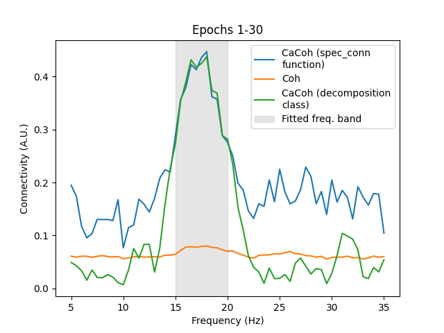
In the above figure, notice also how the CaCoh results from the decomposition class show less connectivity outside of the 15-20 Hz range compared to the CaCoh results of the spectral_connectivity_...() functions.

This shows the risk of overfitting filters to noise in the data, even when no genuine connectivity is present. This problem can be mitigated by fitting filters to only those frequencies where you expect connectivity to be present, e.g. as is done with the decomposition class.

In addition to assessing the validity of the approach, we can also look at the time taken to run the analysis. Doing so, we see that the decomposition class is much faster than the spectral_connectivity_...() functions, thanks to the fact that the filters are fit to a single frequency band and not each frequency bin.

# Show compute times of analyses
print(
    "Time to fit, transform, and compute connectivity (decomposition class): "
    f"{class_duration:.0f} ms"
)
print(
    f"Time to fit, transform, and compute connectivity (spec_conn function): "
    f"{func_duration:.0f} ms"
)

Time to fit, transform, and compute connectivity (decomposition class): 81 ms
Time to fit, transform, and compute connectivity (spec_conn function): 219 ms

Altogether, the decomposition class offers an efficient way to analyse connectivity in a specific frequency band when fitting filters to and transforming a single piece of data.

Case 2: Fitting to and transforming different data

Another way we can use the decomposition class is by taking the filters trained on one piece of data and applying them to another piece of data. Continuing with our simulated data example, we can reuse the CoherencyDecomposition instance we made earlier, as it already contains filters fit on the first 30 epochs of data. We can then apply those filters to the last 30 epochs of data using the transform() method, extracting this same connectivity component.

# Use filters from first 30 epochs to transform data from last 30 epochs
epochs_transformed = cacoh.transform(epochs[N_EPOCHS // 2 :].get_data())

We can now compute connectivity in the last 30 epochs of the transformed data, which for reference we will compare to connectivity computed using the spectral_connectivity_...() functions, as well as bivariate coherence to again demonstrate the signal-to-noise ratio enhancements the multivariate approach offers.

# Fit, transform, and compute connectivity for last 30 epochs using spec_conn function
con_cacoh_30_60_func = spectral_connectivity_epochs(
    epochs[N_EPOCHS // 2 :],
    method="cacoh",
    indices=([seeds], [targets]),
    fmin=5,
    fmax=35,
    rank=([3], [3]),
)

# Compute connectivity for last 30 epochs transformed with filters from first 30 epochs
con_cacoh_30_60_class = spectral_connectivity_epochs(
    epochs_transformed,
    method="coh",
    indices=cacoh.get_transformed_indices(),
    fmin=5,
    fmax=35,
    sfreq=epochs.info["sfreq"],
)

# Compute bivariate connectivity of last 30 epochs for comparison
con_coh_30_60 = spectral_connectivity_epochs(
    epochs[N_EPOCHS // 2 :],
    method="coh",
    indices=seed_target_indices(seeds, targets),
    fmin=5,
    fmax=35,
)

/home/circleci/project/mne_connectivity/spectral/epochs.py:986: RuntimeWarning: There were no Annotations stored in <EpochsArray | 30 events (all good), 0 – 1.99 s (baseline off), ~1.2 MB, data loaded,
 '1': 30>, so metadata was not modified.
  data.add_annotations_to_metadata(overwrite=True)
Connectivity computation...
    computing connectivity for 1 connections
    using t=0.000s..1.990s for estimation (200 points)
    frequencies: 5.0Hz..35.0Hz (61 points)
    Using multitaper spectrum estimation with 7 DPSS windows
    the following metrics will be computed: CaCoh
    computing cross-spectral density for epoch 1
    computing cross-spectral density for epoch 2
    computing cross-spectral density for epoch 3
    computing cross-spectral density for epoch 4
    computing cross-spectral density for epoch 5
    computing cross-spectral density for epoch 6
    computing cross-spectral density for epoch 7
    computing cross-spectral density for epoch 8
    computing cross-spectral density for epoch 9
    computing cross-spectral density for epoch 10
    computing cross-spectral density for epoch 11
    computing cross-spectral density for epoch 12
    computing cross-spectral density for epoch 13
    computing cross-spectral density for epoch 14
    computing cross-spectral density for epoch 15
    computing cross-spectral density for epoch 16
    computing cross-spectral density for epoch 17
    computing cross-spectral density for epoch 18
    computing cross-spectral density for epoch 19
    computing cross-spectral density for epoch 20
    computing cross-spectral density for epoch 21
    computing cross-spectral density for epoch 22
    computing cross-spectral density for epoch 23
    computing cross-spectral density for epoch 24
    computing cross-spectral density for epoch 25
    computing cross-spectral density for epoch 26
    computing cross-spectral density for epoch 27
    computing cross-spectral density for epoch 28
    computing cross-spectral density for epoch 29
    computing cross-spectral density for epoch 30
Computing CaCoh for connection 1 of 1
[Connectivity computation done]
Connectivity computation...
    computing connectivity for 1 connections
    using t=0.000s..1.990s for estimation (200 points)
    frequencies: 5.0Hz..35.0Hz (61 points)
    Using multitaper spectrum estimation with 7 DPSS windows
    the following metrics will be computed: Coherence
    computing cross-spectral density for epoch 1
    computing cross-spectral density for epoch 2
    computing cross-spectral density for epoch 3
    computing cross-spectral density for epoch 4
    computing cross-spectral density for epoch 5
    computing cross-spectral density for epoch 6
    computing cross-spectral density for epoch 7
    computing cross-spectral density for epoch 8
    computing cross-spectral density for epoch 9
    computing cross-spectral density for epoch 10
    computing cross-spectral density for epoch 11
    computing cross-spectral density for epoch 12
    computing cross-spectral density for epoch 13
    computing cross-spectral density for epoch 14
    computing cross-spectral density for epoch 15
    computing cross-spectral density for epoch 16
    computing cross-spectral density for epoch 17
    computing cross-spectral density for epoch 18
    computing cross-spectral density for epoch 19
    computing cross-spectral density for epoch 20
    computing cross-spectral density for epoch 21
    computing cross-spectral density for epoch 22
    computing cross-spectral density for epoch 23
    computing cross-spectral density for epoch 24
    computing cross-spectral density for epoch 25
    computing cross-spectral density for epoch 26
    computing cross-spectral density for epoch 27
    computing cross-spectral density for epoch 28
    computing cross-spectral density for epoch 29
    computing cross-spectral density for epoch 30
[Connectivity computation done]
/home/circleci/project/mne_connectivity/spectral/epochs.py:986: RuntimeWarning: There were no Annotations stored in <EpochsArray | 30 events (all good), 0 – 1.99 s (baseline off), ~1.2 MB, data loaded,
 '1': 30>, so metadata was not modified.
  data.add_annotations_to_metadata(overwrite=True)
Connectivity computation...
    computing connectivity for 150 connections
    using t=0.000s..1.990s for estimation (200 points)
    frequencies: 5.0Hz..35.0Hz (61 points)
    Using multitaper spectrum estimation with 7 DPSS windows
    the following metrics will be computed: Coherence
    computing cross-spectral density for epoch 1
    computing cross-spectral density for epoch 2
    computing cross-spectral density for epoch 3
    computing cross-spectral density for epoch 4
    computing cross-spectral density for epoch 5
    computing cross-spectral density for epoch 6
    computing cross-spectral density for epoch 7
    computing cross-spectral density for epoch 8
    computing cross-spectral density for epoch 9
    computing cross-spectral density for epoch 10
    computing cross-spectral density for epoch 11
    computing cross-spectral density for epoch 12
    computing cross-spectral density for epoch 13
    computing cross-spectral density for epoch 14
    computing cross-spectral density for epoch 15
    computing cross-spectral density for epoch 16
    computing cross-spectral density for epoch 17
    computing cross-spectral density for epoch 18
    computing cross-spectral density for epoch 19
    computing cross-spectral density for epoch 20
    computing cross-spectral density for epoch 21
    computing cross-spectral density for epoch 22
    computing cross-spectral density for epoch 23
    computing cross-spectral density for epoch 24
    computing cross-spectral density for epoch 25
    computing cross-spectral density for epoch 26
    computing cross-spectral density for epoch 27
    computing cross-spectral density for epoch 28
    computing cross-spectral density for epoch 29
    computing cross-spectral density for epoch 30
[Connectivity computation done]

As you can see, the connectivity profile of the transformed data using filters fit on the first 30 epochs is very similar to the connectivity profile when using filters fit on the last 30 epochs itself. This shows that the filters are generalisable, able to extract the same components of connectivity which they were trained on from new data.

# Plot connectivity
ax = plt.subplot(111)
ax.plot(
    con_cacoh_30_60_func.freqs,
    np.abs(con_cacoh_30_60_func.get_data()[0]),
    label="CaCoh (spec_conn\nfunction)",
)
ax.plot(con_coh_30_60.freqs, np.mean(con_coh_30_60.get_data(), axis=0), label="Coh")
ax.plot(
    con_cacoh_30_60_class.freqs,
    np.abs(con_cacoh_30_60_class.get_data()[0]),
    label="CaCoh (decomposition\nclass)",
)
ax.axvspan(FMIN, FMAX, color="grey", alpha=0.2, label="Fitted freq. band")
ax.set_xlabel("Frequency (Hz)")
ax.set_ylabel("Connectivity (A.U.)")
ax.set_title("Epochs 31-60")
plt.legend()
plt.show()

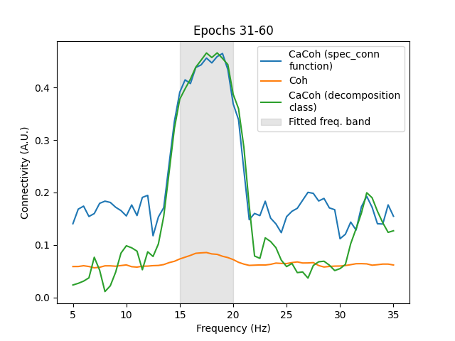
Again, notice how the CaCoh results from the decomposition class show less connectivity outside of the 15-20 Hz range compared to the CaCoh results of the spectral_connectivity_...() functions.

We can also look at the time taken to run the analysis. Below we present a scenario resembling an online sliding window approach typical of a BCI system. We consider the first 30 epochs to be the training data that the filters should be fit to, and the last 30 epochs to be the windows of data that the filters should be applied to, transforming and computing the connectivity of each window (epoch) of data sequentially.

# Instantiate decomposition class
cacoh = CoherencyDecomposition(
    info=epochs.info,
    method="cacoh",
    indices=(seeds, targets),
    mode="multitaper",
    fmin=FMIN,
    fmax=FMAX,
    rank=(3, 3),
)

# Time fitting of filters
start_fit = time.time()
cacoh.fit(epochs[: N_EPOCHS // 2].get_data())
fit_duration = (time.time() - start_fit) * 1000

# Time transforming data of each epoch iteratively
start_transform = time.time()
for epoch in epochs[N_EPOCHS // 2 :]:
    epoch_transformed = cacoh.transform(epoch)
    spectral_connectivity_epochs(
        np.expand_dims(epoch_transformed, axis=0),
        method="coh",
        indices=cacoh.get_transformed_indices(),
        fmin=5,
        fmax=35,
        sfreq=epochs.info["sfreq"],
    )
transform_duration = (time.time() - start_transform) * 1000

    Using multitaper spectrum estimation with 7 DPSS windows
Computing cross-spectral density from epochs...

  0%|          | CSD epoch blocks : 0/30 [00:00<?,       ?it/s]
 30%|███       | CSD epoch blocks : 9/30 [00:00<00:00,  521.95it/s]
 60%|██████    | CSD epoch blocks : 18/30 [00:00<00:00,  528.33it/s]
 90%|█████████ | CSD epoch blocks : 27/30 [00:00<00:00,  535.80it/s]
100%|██████████| CSD epoch blocks : 30/30 [00:00<00:00,  533.35it/s]
[done]
Computing CaCoh for connection 1 of 1
Connectivity computation...
    computing connectivity for 1 connections
    using t=0.000s..1.990s for estimation (200 points)
    frequencies: 5.0Hz..35.0Hz (61 points)
    Using multitaper spectrum estimation with 7 DPSS windows
    the following metrics will be computed: Coherence
    computing cross-spectral density for epoch 1
[Connectivity computation done]
Connectivity computation...
    computing connectivity for 1 connections
    using t=0.000s..1.990s for estimation (200 points)
    frequencies: 5.0Hz..35.0Hz (61 points)
    Using multitaper spectrum estimation with 7 DPSS windows
    the following metrics will be computed: Coherence
    computing cross-spectral density for epoch 1
[Connectivity computation done]
Connectivity computation...
    computing connectivity for 1 connections
    using t=0.000s..1.990s for estimation (200 points)
    frequencies: 5.0Hz..35.0Hz (61 points)
    Using multitaper spectrum estimation with 7 DPSS windows
    the following metrics will be computed: Coherence
    computing cross-spectral density for epoch 1
[Connectivity computation done]
Connectivity computation...
    computing connectivity for 1 connections
    using t=0.000s..1.990s for estimation (200 points)
    frequencies: 5.0Hz..35.0Hz (61 points)
    Using multitaper spectrum estimation with 7 DPSS windows
    the following metrics will be computed: Coherence
    computing cross-spectral density for epoch 1
[Connectivity computation done]
Connectivity computation...
    computing connectivity for 1 connections
    using t=0.000s..1.990s for estimation (200 points)
    frequencies: 5.0Hz..35.0Hz (61 points)
    Using multitaper spectrum estimation with 7 DPSS windows
    the following metrics will be computed: Coherence
    computing cross-spectral density for epoch 1
[Connectivity computation done]
Connectivity computation...
    computing connectivity for 1 connections
    using t=0.000s..1.990s for estimation (200 points)
    frequencies: 5.0Hz..35.0Hz (61 points)
    Using multitaper spectrum estimation with 7 DPSS windows
    the following metrics will be computed: Coherence
    computing cross-spectral density for epoch 1
[Connectivity computation done]
Connectivity computation...
    computing connectivity for 1 connections
    using t=0.000s..1.990s for estimation (200 points)
    frequencies: 5.0Hz..35.0Hz (61 points)
    Using multitaper spectrum estimation with 7 DPSS windows
    the following metrics will be computed: Coherence
    computing cross-spectral density for epoch 1
[Connectivity computation done]
Connectivity computation...
    computing connectivity for 1 connections
    using t=0.000s..1.990s for estimation (200 points)
    frequencies: 5.0Hz..35.0Hz (61 points)
    Using multitaper spectrum estimation with 7 DPSS windows
    the following metrics will be computed: Coherence
    computing cross-spectral density for epoch 1
[Connectivity computation done]
Connectivity computation...
    computing connectivity for 1 connections
    using t=0.000s..1.990s for estimation (200 points)
    frequencies: 5.0Hz..35.0Hz (61 points)
    Using multitaper spectrum estimation with 7 DPSS windows
    the following metrics will be computed: Coherence
    computing cross-spectral density for epoch 1
[Connectivity computation done]
Connectivity computation...
    computing connectivity for 1 connections
    using t=0.000s..1.990s for estimation (200 points)
    frequencies: 5.0Hz..35.0Hz (61 points)
    Using multitaper spectrum estimation with 7 DPSS windows
    the following metrics will be computed: Coherence
    computing cross-spectral density for epoch 1
[Connectivity computation done]
Connectivity computation...
    computing connectivity for 1 connections
    using t=0.000s..1.990s for estimation (200 points)
    frequencies: 5.0Hz..35.0Hz (61 points)
    Using multitaper spectrum estimation with 7 DPSS windows
    the following metrics will be computed: Coherence
    computing cross-spectral density for epoch 1
[Connectivity computation done]
Connectivity computation...
    computing connectivity for 1 connections
    using t=0.000s..1.990s for estimation (200 points)
    frequencies: 5.0Hz..35.0Hz (61 points)
    Using multitaper spectrum estimation with 7 DPSS windows
    the following metrics will be computed: Coherence
    computing cross-spectral density for epoch 1
[Connectivity computation done]
Connectivity computation...
    computing connectivity for 1 connections
    using t=0.000s..1.990s for estimation (200 points)
    frequencies: 5.0Hz..35.0Hz (61 points)
    Using multitaper spectrum estimation with 7 DPSS windows
    the following metrics will be computed: Coherence
    computing cross-spectral density for epoch 1
[Connectivity computation done]
Connectivity computation...
    computing connectivity for 1 connections
    using t=0.000s..1.990s for estimation (200 points)
    frequencies: 5.0Hz..35.0Hz (61 points)
    Using multitaper spectrum estimation with 7 DPSS windows
    the following metrics will be computed: Coherence
    computing cross-spectral density for epoch 1
[Connectivity computation done]
Connectivity computation...
    computing connectivity for 1 connections
    using t=0.000s..1.990s for estimation (200 points)
    frequencies: 5.0Hz..35.0Hz (61 points)
    Using multitaper spectrum estimation with 7 DPSS windows
    the following metrics will be computed: Coherence
    computing cross-spectral density for epoch 1
[Connectivity computation done]
Connectivity computation...
    computing connectivity for 1 connections
    using t=0.000s..1.990s for estimation (200 points)
    frequencies: 5.0Hz..35.0Hz (61 points)
    Using multitaper spectrum estimation with 7 DPSS windows
    the following metrics will be computed: Coherence
    computing cross-spectral density for epoch 1
[Connectivity computation done]
Connectivity computation...
    computing connectivity for 1 connections
    using t=0.000s..1.990s for estimation (200 points)
    frequencies: 5.0Hz..35.0Hz (61 points)
    Using multitaper spectrum estimation with 7 DPSS windows
    the following metrics will be computed: Coherence
    computing cross-spectral density for epoch 1
[Connectivity computation done]
Connectivity computation...
    computing connectivity for 1 connections
    using t=0.000s..1.990s for estimation (200 points)
    frequencies: 5.0Hz..35.0Hz (61 points)
    Using multitaper spectrum estimation with 7 DPSS windows
    the following metrics will be computed: Coherence
    computing cross-spectral density for epoch 1
[Connectivity computation done]
Connectivity computation...
    computing connectivity for 1 connections
    using t=0.000s..1.990s for estimation (200 points)
    frequencies: 5.0Hz..35.0Hz (61 points)
    Using multitaper spectrum estimation with 7 DPSS windows
    the following metrics will be computed: Coherence
    computing cross-spectral density for epoch 1
[Connectivity computation done]
Connectivity computation...
    computing connectivity for 1 connections
    using t=0.000s..1.990s for estimation (200 points)
    frequencies: 5.0Hz..35.0Hz (61 points)
    Using multitaper spectrum estimation with 7 DPSS windows
    the following metrics will be computed: Coherence
    computing cross-spectral density for epoch 1
[Connectivity computation done]
Connectivity computation...
    computing connectivity for 1 connections
    using t=0.000s..1.990s for estimation (200 points)
    frequencies: 5.0Hz..35.0Hz (61 points)
    Using multitaper spectrum estimation with 7 DPSS windows
    the following metrics will be computed: Coherence
    computing cross-spectral density for epoch 1
[Connectivity computation done]
Connectivity computation...
    computing connectivity for 1 connections
    using t=0.000s..1.990s for estimation (200 points)
    frequencies: 5.0Hz..35.0Hz (61 points)
    Using multitaper spectrum estimation with 7 DPSS windows
    the following metrics will be computed: Coherence
    computing cross-spectral density for epoch 1
[Connectivity computation done]
Connectivity computation...
    computing connectivity for 1 connections
    using t=0.000s..1.990s for estimation (200 points)
    frequencies: 5.0Hz..35.0Hz (61 points)
    Using multitaper spectrum estimation with 7 DPSS windows
    the following metrics will be computed: Coherence
    computing cross-spectral density for epoch 1
[Connectivity computation done]
Connectivity computation...
    computing connectivity for 1 connections
    using t=0.000s..1.990s for estimation (200 points)
    frequencies: 5.0Hz..35.0Hz (61 points)
    Using multitaper spectrum estimation with 7 DPSS windows
    the following metrics will be computed: Coherence
    computing cross-spectral density for epoch 1
[Connectivity computation done]
Connectivity computation...
    computing connectivity for 1 connections
    using t=0.000s..1.990s for estimation (200 points)
    frequencies: 5.0Hz..35.0Hz (61 points)
    Using multitaper spectrum estimation with 7 DPSS windows
    the following metrics will be computed: Coherence
    computing cross-spectral density for epoch 1
[Connectivity computation done]
Connectivity computation...
    computing connectivity for 1 connections
    using t=0.000s..1.990s for estimation (200 points)
    frequencies: 5.0Hz..35.0Hz (61 points)
    Using multitaper spectrum estimation with 7 DPSS windows
    the following metrics will be computed: Coherence
    computing cross-spectral density for epoch 1
[Connectivity computation done]
Connectivity computation...
    computing connectivity for 1 connections
    using t=0.000s..1.990s for estimation (200 points)
    frequencies: 5.0Hz..35.0Hz (61 points)
    Using multitaper spectrum estimation with 7 DPSS windows
    the following metrics will be computed: Coherence
    computing cross-spectral density for epoch 1
[Connectivity computation done]
Connectivity computation...
    computing connectivity for 1 connections
    using t=0.000s..1.990s for estimation (200 points)
    frequencies: 5.0Hz..35.0Hz (61 points)
    Using multitaper spectrum estimation with 7 DPSS windows
    the following metrics will be computed: Coherence
    computing cross-spectral density for epoch 1
[Connectivity computation done]
Connectivity computation...
    computing connectivity for 1 connections
    using t=0.000s..1.990s for estimation (200 points)
    frequencies: 5.0Hz..35.0Hz (61 points)
    Using multitaper spectrum estimation with 7 DPSS windows
    the following metrics will be computed: Coherence
    computing cross-spectral density for epoch 1
[Connectivity computation done]
Connectivity computation...
    computing connectivity for 1 connections
    using t=0.000s..1.990s for estimation (200 points)
    frequencies: 5.0Hz..35.0Hz (61 points)
    Using multitaper spectrum estimation with 7 DPSS windows
    the following metrics will be computed: Coherence
    computing cross-spectral density for epoch 1
[Connectivity computation done]

Doing so, we see that once the filters have been fit, it takes only a few milliseconds to transform each window of data and compute its connectivity.

# Show compute times of decomposition class
print(f"Time to fit filters: {fit_duration:.0f} ms")
print(f"Time to transform data and compute connectivity: {transform_duration:.0f} ms")
print(f"Total time: {fit_duration + transform_duration:.0f} ms")

print(
    "\nTime to transform data and compute connectivity per epoch (window): ",
    f"{transform_duration/(N_EPOCHS//2):.0f} ms",
)

Time to fit filters: 65 ms
Time to transform data and compute connectivity: 117 ms
Total time: 182 ms

Time to transform data and compute connectivity per epoch (window):  4 ms

In contrast, here we follow the same sequential window approach, but fit filters to each window separately rather than using a pre-computed set.

# Time fitting and transforming data of each epoch iteratively
start_fit_transform = time.time()
for epoch in epochs[N_EPOCHS // 2 :]:
    spectral_connectivity_epochs(
        np.expand_dims(epoch, axis=0),
        method="cacoh",
        indices=([seeds], [targets]),
        fmin=5,
        fmax=35,
        sfreq=epochs.info["sfreq"],
        rank=([3], [3]),
    )
fit_transform_duration = (time.time() - start_fit_transform) * 1000

Connectivity computation...
    computing connectivity for 1 connections
    using t=0.000s..1.990s for estimation (200 points)
    frequencies: 5.0Hz..35.0Hz (61 points)
    Using multitaper spectrum estimation with 7 DPSS windows
    the following metrics will be computed: CaCoh
    computing cross-spectral density for epoch 1
Computing CaCoh for connection 1 of 1
[Connectivity computation done]
Connectivity computation...
    computing connectivity for 1 connections
    using t=0.000s..1.990s for estimation (200 points)
    frequencies: 5.0Hz..35.0Hz (61 points)
    Using multitaper spectrum estimation with 7 DPSS windows
    the following metrics will be computed: CaCoh
    computing cross-spectral density for epoch 1
Computing CaCoh for connection 1 of 1
[Connectivity computation done]
Connectivity computation...
    computing connectivity for 1 connections
    using t=0.000s..1.990s for estimation (200 points)
    frequencies: 5.0Hz..35.0Hz (61 points)
    Using multitaper spectrum estimation with 7 DPSS windows
    the following metrics will be computed: CaCoh
    computing cross-spectral density for epoch 1
Computing CaCoh for connection 1 of 1
[Connectivity computation done]
Connectivity computation...
    computing connectivity for 1 connections
    using t=0.000s..1.990s for estimation (200 points)
    frequencies: 5.0Hz..35.0Hz (61 points)
    Using multitaper spectrum estimation with 7 DPSS windows
    the following metrics will be computed: CaCoh
    computing cross-spectral density for epoch 1
Computing CaCoh for connection 1 of 1
[Connectivity computation done]
Connectivity computation...
    computing connectivity for 1 connections
    using t=0.000s..1.990s for estimation (200 points)
    frequencies: 5.0Hz..35.0Hz (61 points)
    Using multitaper spectrum estimation with 7 DPSS windows
    the following metrics will be computed: CaCoh
    computing cross-spectral density for epoch 1
Computing CaCoh for connection 1 of 1
[Connectivity computation done]
Connectivity computation...
    computing connectivity for 1 connections
    using t=0.000s..1.990s for estimation (200 points)
    frequencies: 5.0Hz..35.0Hz (61 points)
    Using multitaper spectrum estimation with 7 DPSS windows
    the following metrics will be computed: CaCoh
    computing cross-spectral density for epoch 1
Computing CaCoh for connection 1 of 1
[Connectivity computation done]
Connectivity computation...
    computing connectivity for 1 connections
    using t=0.000s..1.990s for estimation (200 points)
    frequencies: 5.0Hz..35.0Hz (61 points)
    Using multitaper spectrum estimation with 7 DPSS windows
    the following metrics will be computed: CaCoh
    computing cross-spectral density for epoch 1
Computing CaCoh for connection 1 of 1
[Connectivity computation done]
Connectivity computation...
    computing connectivity for 1 connections
    using t=0.000s..1.990s for estimation (200 points)
    frequencies: 5.0Hz..35.0Hz (61 points)
    Using multitaper spectrum estimation with 7 DPSS windows
    the following metrics will be computed: CaCoh
    computing cross-spectral density for epoch 1
Computing CaCoh for connection 1 of 1
[Connectivity computation done]
Connectivity computation...
    computing connectivity for 1 connections
    using t=0.000s..1.990s for estimation (200 points)
    frequencies: 5.0Hz..35.0Hz (61 points)
    Using multitaper spectrum estimation with 7 DPSS windows
    the following metrics will be computed: CaCoh
    computing cross-spectral density for epoch 1
Computing CaCoh for connection 1 of 1
[Connectivity computation done]
Connectivity computation...
    computing connectivity for 1 connections
    using t=0.000s..1.990s for estimation (200 points)
    frequencies: 5.0Hz..35.0Hz (61 points)
    Using multitaper spectrum estimation with 7 DPSS windows
    the following metrics will be computed: CaCoh
    computing cross-spectral density for epoch 1
Computing CaCoh for connection 1 of 1
[Connectivity computation done]
Connectivity computation...
    computing connectivity for 1 connections
    using t=0.000s..1.990s for estimation (200 points)
    frequencies: 5.0Hz..35.0Hz (61 points)
    Using multitaper spectrum estimation with 7 DPSS windows
    the following metrics will be computed: CaCoh
    computing cross-spectral density for epoch 1
Computing CaCoh for connection 1 of 1
[Connectivity computation done]
Connectivity computation...
    computing connectivity for 1 connections
    using t=0.000s..1.990s for estimation (200 points)
    frequencies: 5.0Hz..35.0Hz (61 points)
    Using multitaper spectrum estimation with 7 DPSS windows
    the following metrics will be computed: CaCoh
    computing cross-spectral density for epoch 1
Computing CaCoh for connection 1 of 1
[Connectivity computation done]
Connectivity computation...
    computing connectivity for 1 connections
    using t=0.000s..1.990s for estimation (200 points)
    frequencies: 5.0Hz..35.0Hz (61 points)
    Using multitaper spectrum estimation with 7 DPSS windows
    the following metrics will be computed: CaCoh
    computing cross-spectral density for epoch 1
Computing CaCoh for connection 1 of 1
[Connectivity computation done]
Connectivity computation...
    computing connectivity for 1 connections
    using t=0.000s..1.990s for estimation (200 points)
    frequencies: 5.0Hz..35.0Hz (61 points)
    Using multitaper spectrum estimation with 7 DPSS windows
    the following metrics will be computed: CaCoh
    computing cross-spectral density for epoch 1
Computing CaCoh for connection 1 of 1
[Connectivity computation done]
Connectivity computation...
    computing connectivity for 1 connections
    using t=0.000s..1.990s for estimation (200 points)
    frequencies: 5.0Hz..35.0Hz (61 points)
    Using multitaper spectrum estimation with 7 DPSS windows
    the following metrics will be computed: CaCoh
    computing cross-spectral density for epoch 1
Computing CaCoh for connection 1 of 1
[Connectivity computation done]
Connectivity computation...
    computing connectivity for 1 connections
    using t=0.000s..1.990s for estimation (200 points)
    frequencies: 5.0Hz..35.0Hz (61 points)
    Using multitaper spectrum estimation with 7 DPSS windows
    the following metrics will be computed: CaCoh
    computing cross-spectral density for epoch 1
Computing CaCoh for connection 1 of 1
[Connectivity computation done]
Connectivity computation...
    computing connectivity for 1 connections
    using t=0.000s..1.990s for estimation (200 points)
    frequencies: 5.0Hz..35.0Hz (61 points)
    Using multitaper spectrum estimation with 7 DPSS windows
    the following metrics will be computed: CaCoh
    computing cross-spectral density for epoch 1
Computing CaCoh for connection 1 of 1
[Connectivity computation done]
Connectivity computation...
    computing connectivity for 1 connections
    using t=0.000s..1.990s for estimation (200 points)
    frequencies: 5.0Hz..35.0Hz (61 points)
    Using multitaper spectrum estimation with 7 DPSS windows
    the following metrics will be computed: CaCoh
    computing cross-spectral density for epoch 1
Computing CaCoh for connection 1 of 1
[Connectivity computation done]
Connectivity computation...
    computing connectivity for 1 connections
    using t=0.000s..1.990s for estimation (200 points)
    frequencies: 5.0Hz..35.0Hz (61 points)
    Using multitaper spectrum estimation with 7 DPSS windows
    the following metrics will be computed: CaCoh
    computing cross-spectral density for epoch 1
Computing CaCoh for connection 1 of 1
[Connectivity computation done]
Connectivity computation...
    computing connectivity for 1 connections
    using t=0.000s..1.990s for estimation (200 points)
    frequencies: 5.0Hz..35.0Hz (61 points)
    Using multitaper spectrum estimation with 7 DPSS windows
    the following metrics will be computed: CaCoh
    computing cross-spectral density for epoch 1
Computing CaCoh for connection 1 of 1
[Connectivity computation done]
Connectivity computation...
    computing connectivity for 1 connections
    using t=0.000s..1.990s for estimation (200 points)
    frequencies: 5.0Hz..35.0Hz (61 points)
    Using multitaper spectrum estimation with 7 DPSS windows
    the following metrics will be computed: CaCoh
    computing cross-spectral density for epoch 1
Computing CaCoh for connection 1 of 1
[Connectivity computation done]
Connectivity computation...
    computing connectivity for 1 connections
    using t=0.000s..1.990s for estimation (200 points)
    frequencies: 5.0Hz..35.0Hz (61 points)
    Using multitaper spectrum estimation with 7 DPSS windows
    the following metrics will be computed: CaCoh
    computing cross-spectral density for epoch 1
Computing CaCoh for connection 1 of 1
[Connectivity computation done]
Connectivity computation...
    computing connectivity for 1 connections
    using t=0.000s..1.990s for estimation (200 points)
    frequencies: 5.0Hz..35.0Hz (61 points)
    Using multitaper spectrum estimation with 7 DPSS windows
    the following metrics will be computed: CaCoh
    computing cross-spectral density for epoch 1
Computing CaCoh for connection 1 of 1
[Connectivity computation done]
Connectivity computation...
    computing connectivity for 1 connections
    using t=0.000s..1.990s for estimation (200 points)
    frequencies: 5.0Hz..35.0Hz (61 points)
    Using multitaper spectrum estimation with 7 DPSS windows
    the following metrics will be computed: CaCoh
    computing cross-spectral density for epoch 1
Computing CaCoh for connection 1 of 1
[Connectivity computation done]
Connectivity computation...
    computing connectivity for 1 connections
    using t=0.000s..1.990s for estimation (200 points)
    frequencies: 5.0Hz..35.0Hz (61 points)
    Using multitaper spectrum estimation with 7 DPSS windows
    the following metrics will be computed: CaCoh
    computing cross-spectral density for epoch 1
Computing CaCoh for connection 1 of 1
[Connectivity computation done]
Connectivity computation...
    computing connectivity for 1 connections
    using t=0.000s..1.990s for estimation (200 points)
    frequencies: 5.0Hz..35.0Hz (61 points)
    Using multitaper spectrum estimation with 7 DPSS windows
    the following metrics will be computed: CaCoh
    computing cross-spectral density for epoch 1
Computing CaCoh for connection 1 of 1
[Connectivity computation done]
Connectivity computation...
    computing connectivity for 1 connections
    using t=0.000s..1.990s for estimation (200 points)
    frequencies: 5.0Hz..35.0Hz (61 points)
    Using multitaper spectrum estimation with 7 DPSS windows
    the following metrics will be computed: CaCoh
    computing cross-spectral density for epoch 1
Computing CaCoh for connection 1 of 1
[Connectivity computation done]
Connectivity computation...
    computing connectivity for 1 connections
    using t=0.000s..1.990s for estimation (200 points)
    frequencies: 5.0Hz..35.0Hz (61 points)
    Using multitaper spectrum estimation with 7 DPSS windows
    the following metrics will be computed: CaCoh
    computing cross-spectral density for epoch 1
Computing CaCoh for connection 1 of 1
[Connectivity computation done]
Connectivity computation...
    computing connectivity for 1 connections
    using t=0.000s..1.990s for estimation (200 points)
    frequencies: 5.0Hz..35.0Hz (61 points)
    Using multitaper spectrum estimation with 7 DPSS windows
    the following metrics will be computed: CaCoh
    computing cross-spectral density for epoch 1
Computing CaCoh for connection 1 of 1
[Connectivity computation done]
Connectivity computation...
    computing connectivity for 1 connections
    using t=0.000s..1.990s for estimation (200 points)
    frequencies: 5.0Hz..35.0Hz (61 points)
    Using multitaper spectrum estimation with 7 DPSS windows
    the following metrics will be computed: CaCoh
    computing cross-spectral density for epoch 1
Computing CaCoh for connection 1 of 1
[Connectivity computation done]

Naturally, the process of fitting and transforming the data for each window is considerably slower.

# Show compute times of spec_conn function
print(
    f"Time to fit, transform, and compute connectivity: {fit_transform_duration:.0f} ms"
)

print(
    "\nTime to fit, transform, and compute connectivity per epoch (window): ",
    f"{fit_transform_duration/(N_EPOCHS//2):.0f} ms",
)

Time to fit, transform, and compute connectivity: 891 ms

Time to fit, transform, and compute connectivity per epoch (window):  30 ms

Furthermore, given the noisy nature of single windows of data, there is a risk of overfitting the filters to this noise as opposed to the genuine interaction(s) of interest. This risk is mitigated by performing the initial filter fitting on a larger set of data.

As a side note, it is important to consider that a multivariate approach may be as fast or even faster than a bivariate approach, depending on the number of connections and degree of rank subspace projection being performed.

# Time transforming data of each epoch iteratively
start = time.time()
for epoch in epochs[N_EPOCHS // 2 :]:
    spectral_connectivity_epochs(
        np.expand_dims(epoch, axis=0),
        method="coh",
        indices=seed_target_indices(seeds, targets),
        fmin=5,
        fmax=35,
        sfreq=epochs.info["sfreq"],
    )
duration = (time.time() - start) * 1000

Connectivity computation...
    computing connectivity for 150 connections
    using t=0.000s..1.990s for estimation (200 points)
    frequencies: 5.0Hz..35.0Hz (61 points)
    Using multitaper spectrum estimation with 7 DPSS windows
    the following metrics will be computed: Coherence
    computing cross-spectral density for epoch 1
[Connectivity computation done]
Connectivity computation...
    computing connectivity for 150 connections
    using t=0.000s..1.990s for estimation (200 points)
    frequencies: 5.0Hz..35.0Hz (61 points)
    Using multitaper spectrum estimation with 7 DPSS windows
    the following metrics will be computed: Coherence
    computing cross-spectral density for epoch 1
[Connectivity computation done]
Connectivity computation...
    computing connectivity for 150 connections
    using t=0.000s..1.990s for estimation (200 points)
    frequencies: 5.0Hz..35.0Hz (61 points)
    Using multitaper spectrum estimation with 7 DPSS windows
    the following metrics will be computed: Coherence
    computing cross-spectral density for epoch 1
[Connectivity computation done]
Connectivity computation...
    computing connectivity for 150 connections
    using t=0.000s..1.990s for estimation (200 points)
    frequencies: 5.0Hz..35.0Hz (61 points)
    Using multitaper spectrum estimation with 7 DPSS windows
    the following metrics will be computed: Coherence
    computing cross-spectral density for epoch 1
[Connectivity computation done]
Connectivity computation...
    computing connectivity for 150 connections
    using t=0.000s..1.990s for estimation (200 points)
    frequencies: 5.0Hz..35.0Hz (61 points)
    Using multitaper spectrum estimation with 7 DPSS windows
    the following metrics will be computed: Coherence
    computing cross-spectral density for epoch 1
[Connectivity computation done]
Connectivity computation...
    computing connectivity for 150 connections
    using t=0.000s..1.990s for estimation (200 points)
    frequencies: 5.0Hz..35.0Hz (61 points)
    Using multitaper spectrum estimation with 7 DPSS windows
    the following metrics will be computed: Coherence
    computing cross-spectral density for epoch 1
[Connectivity computation done]
Connectivity computation...
    computing connectivity for 150 connections
    using t=0.000s..1.990s for estimation (200 points)
    frequencies: 5.0Hz..35.0Hz (61 points)
    Using multitaper spectrum estimation with 7 DPSS windows
    the following metrics will be computed: Coherence
    computing cross-spectral density for epoch 1
[Connectivity computation done]
Connectivity computation...
    computing connectivity for 150 connections
    using t=0.000s..1.990s for estimation (200 points)
    frequencies: 5.0Hz..35.0Hz (61 points)
    Using multitaper spectrum estimation with 7 DPSS windows
    the following metrics will be computed: Coherence
    computing cross-spectral density for epoch 1
[Connectivity computation done]
Connectivity computation...
    computing connectivity for 150 connections
    using t=0.000s..1.990s for estimation (200 points)
    frequencies: 5.0Hz..35.0Hz (61 points)
    Using multitaper spectrum estimation with 7 DPSS windows
    the following metrics will be computed: Coherence
    computing cross-spectral density for epoch 1
[Connectivity computation done]
Connectivity computation...
    computing connectivity for 150 connections
    using t=0.000s..1.990s for estimation (200 points)
    frequencies: 5.0Hz..35.0Hz (61 points)
    Using multitaper spectrum estimation with 7 DPSS windows
    the following metrics will be computed: Coherence
    computing cross-spectral density for epoch 1
[Connectivity computation done]
Connectivity computation...
    computing connectivity for 150 connections
    using t=0.000s..1.990s for estimation (200 points)
    frequencies: 5.0Hz..35.0Hz (61 points)
    Using multitaper spectrum estimation with 7 DPSS windows
    the following metrics will be computed: Coherence
    computing cross-spectral density for epoch 1
[Connectivity computation done]
Connectivity computation...
    computing connectivity for 150 connections
    using t=0.000s..1.990s for estimation (200 points)
    frequencies: 5.0Hz..35.0Hz (61 points)
    Using multitaper spectrum estimation with 7 DPSS windows
    the following metrics will be computed: Coherence
    computing cross-spectral density for epoch 1
[Connectivity computation done]
Connectivity computation...
    computing connectivity for 150 connections
    using t=0.000s..1.990s for estimation (200 points)
    frequencies: 5.0Hz..35.0Hz (61 points)
    Using multitaper spectrum estimation with 7 DPSS windows
    the following metrics will be computed: Coherence
    computing cross-spectral density for epoch 1
[Connectivity computation done]
Connectivity computation...
    computing connectivity for 150 connections
    using t=0.000s..1.990s for estimation (200 points)
    frequencies: 5.0Hz..35.0Hz (61 points)
    Using multitaper spectrum estimation with 7 DPSS windows
    the following metrics will be computed: Coherence
    computing cross-spectral density for epoch 1
[Connectivity computation done]
Connectivity computation...
    computing connectivity for 150 connections
    using t=0.000s..1.990s for estimation (200 points)
    frequencies: 5.0Hz..35.0Hz (61 points)
    Using multitaper spectrum estimation with 7 DPSS windows
    the following metrics will be computed: Coherence
    computing cross-spectral density for epoch 1
[Connectivity computation done]
Connectivity computation...
    computing connectivity for 150 connections
    using t=0.000s..1.990s for estimation (200 points)
    frequencies: 5.0Hz..35.0Hz (61 points)
    Using multitaper spectrum estimation with 7 DPSS windows
    the following metrics will be computed: Coherence
    computing cross-spectral density for epoch 1
[Connectivity computation done]
Connectivity computation...
    computing connectivity for 150 connections
    using t=0.000s..1.990s for estimation (200 points)
    frequencies: 5.0Hz..35.0Hz (61 points)
    Using multitaper spectrum estimation with 7 DPSS windows
    the following metrics will be computed: Coherence
    computing cross-spectral density for epoch 1
[Connectivity computation done]
Connectivity computation...
    computing connectivity for 150 connections
    using t=0.000s..1.990s for estimation (200 points)
    frequencies: 5.0Hz..35.0Hz (61 points)
    Using multitaper spectrum estimation with 7 DPSS windows
    the following metrics will be computed: Coherence
    computing cross-spectral density for epoch 1
[Connectivity computation done]
Connectivity computation...
    computing connectivity for 150 connections
    using t=0.000s..1.990s for estimation (200 points)
    frequencies: 5.0Hz..35.0Hz (61 points)
    Using multitaper spectrum estimation with 7 DPSS windows
    the following metrics will be computed: Coherence
    computing cross-spectral density for epoch 1
[Connectivity computation done]
Connectivity computation...
    computing connectivity for 150 connections
    using t=0.000s..1.990s for estimation (200 points)
    frequencies: 5.0Hz..35.0Hz (61 points)
    Using multitaper spectrum estimation with 7 DPSS windows
    the following metrics will be computed: Coherence
    computing cross-spectral density for epoch 1
[Connectivity computation done]
Connectivity computation...
    computing connectivity for 150 connections
    using t=0.000s..1.990s for estimation (200 points)
    frequencies: 5.0Hz..35.0Hz (61 points)
    Using multitaper spectrum estimation with 7 DPSS windows
    the following metrics will be computed: Coherence
    computing cross-spectral density for epoch 1
[Connectivity computation done]
Connectivity computation...
    computing connectivity for 150 connections
    using t=0.000s..1.990s for estimation (200 points)
    frequencies: 5.0Hz..35.0Hz (61 points)
    Using multitaper spectrum estimation with 7 DPSS windows
    the following metrics will be computed: Coherence
    computing cross-spectral density for epoch 1
[Connectivity computation done]
Connectivity computation...
    computing connectivity for 150 connections
    using t=0.000s..1.990s for estimation (200 points)
    frequencies: 5.0Hz..35.0Hz (61 points)
    Using multitaper spectrum estimation with 7 DPSS windows
    the following metrics will be computed: Coherence
    computing cross-spectral density for epoch 1
[Connectivity computation done]
Connectivity computation...
    computing connectivity for 150 connections
    using t=0.000s..1.990s for estimation (200 points)
    frequencies: 5.0Hz..35.0Hz (61 points)
    Using multitaper spectrum estimation with 7 DPSS windows
    the following metrics will be computed: Coherence
    computing cross-spectral density for epoch 1
[Connectivity computation done]
Connectivity computation...
    computing connectivity for 150 connections
    using t=0.000s..1.990s for estimation (200 points)
    frequencies: 5.0Hz..35.0Hz (61 points)
    Using multitaper spectrum estimation with 7 DPSS windows
    the following metrics will be computed: Coherence
    computing cross-spectral density for epoch 1
[Connectivity computation done]
Connectivity computation...
    computing connectivity for 150 connections
    using t=0.000s..1.990s for estimation (200 points)
    frequencies: 5.0Hz..35.0Hz (61 points)
    Using multitaper spectrum estimation with 7 DPSS windows
    the following metrics will be computed: Coherence
    computing cross-spectral density for epoch 1
[Connectivity computation done]
Connectivity computation...
    computing connectivity for 150 connections
    using t=0.000s..1.990s for estimation (200 points)
    frequencies: 5.0Hz..35.0Hz (61 points)
    Using multitaper spectrum estimation with 7 DPSS windows
    the following metrics will be computed: Coherence
    computing cross-spectral density for epoch 1
[Connectivity computation done]
Connectivity computation...
    computing connectivity for 150 connections
    using t=0.000s..1.990s for estimation (200 points)
    frequencies: 5.0Hz..35.0Hz (61 points)
    Using multitaper spectrum estimation with 7 DPSS windows
    the following metrics will be computed: Coherence
    computing cross-spectral density for epoch 1
[Connectivity computation done]
Connectivity computation...
    computing connectivity for 150 connections
    using t=0.000s..1.990s for estimation (200 points)
    frequencies: 5.0Hz..35.0Hz (61 points)
    Using multitaper spectrum estimation with 7 DPSS windows
    the following metrics will be computed: Coherence
    computing cross-spectral density for epoch 1
[Connectivity computation done]
Connectivity computation...
    computing connectivity for 150 connections
    using t=0.000s..1.990s for estimation (200 points)
    frequencies: 5.0Hz..35.0Hz (61 points)
    Using multitaper spectrum estimation with 7 DPSS windows
    the following metrics will be computed: Coherence
    computing cross-spectral density for epoch 1
[Connectivity computation done]

In this instance, the standard bivariate approach is slower than the decomposition class approach above.

# Show compute times of bivariate connectivity
print(f"Time to compute connectivity: {duration:.0f} ms")

print(
    "\nTime to compute connectivity per epoch (window): ",
    f"{duration/(N_EPOCHS//2):.0f} ms",
)

Time to compute connectivity: 172 ms

Time to compute connectivity per epoch (window):  6 ms

Altogether, the decomposition class also offers an efficient way to analyse connectivity in a specific frequency band when fitting filters to one piece of data and transforming other pieces of data.

Component specificity of filters

We have spoken much about how the filters extract particular components of connectivity, which we elaborate on here. The filters act as spatial weights, controlling how much each channel contributes to the given connectivity component. Although we fit these filters to a specific frequency band, they do not operate in a frequency-specific manner.

For example, say you have two sets of data: Data 1 with an interaction at 15-20 Hz; and Data 2 with an interaction at 5-10 Hz. We fit the filters at 15-20 Hz to Data 1, and apply the filters to Data 2.

If the connectivity components in Data 1 and Data 2 have different spatial distributions (i.e. different channels contribute to connectivity in each set of data), the filters fit to 15-20 Hz on Data 1 will not extract the 5-10 Hz connectivity from Data 2.

On the other hand, if the connectivity components in Data 1 and Data 2 have the same spatial distribution (i.e. the same channels contribute to connectivity in both sets of data), the filters fit to 15-20 Hz on Data 1 will extract the 5-10 Hz connectivity from Data 2. Because of this, it is generally recommended that you only consider the connectivity results for those frequencies where you originally fit the filters.

Furthermore, if Data 1 and Data 2 both have interactions at the same frequency band (e.g. 15-20 Hz) but with different spatial distributions, the filters fit to 15-20 Hz on Data 1 will not extract the 15-20 Hz connectivity from Data 2. This is because the filters extract connectivity components according to particular spatial distributions, and if the spatial distributions differ, these interactions are by definition distinct components, even if they occur at the same frequencies.

Limitations

Finally, it is important to discuss a key limitation of the decoding module approach: the need to define a specific frequency band. Defining this band requires some existing knowledge about your data or the oscillatory activity you are studying. This insight may come from a pilot study where a frequency band of interest was identified, a canonical frequency band defined in the literature, etc… In contrast, by fitting filters to each frequency bin, the standard spectral_connectivity_...() functions are more data-driven.

Additionally, by applying filters fit on one set of data to another, you are assuming that the connectivity components the filters are designed to extract are consistent across the two sets of data. However, this may not be the case if you are applying the filters to data from a distinct functional state where the spatial distribution of the components differs. Again, by fitting filters to each new set of data passed in, the standard spectral_connectivity_...() functions are more data-driven, extracting whatever connectivity components are present in that data.

On these points, we note that the spectral_connectivity_...() functions complement the decoding module classes well, offering a tool by which to explore your data to: identify possible frequency bands of interest; and identify the spatial distributions of connectivity components to determine if they are consistent across different portions of the data.

Ultimately, there are distinct advantages and disadvantages to both approaches, and one may be more suitable than the other depending on your use case.

References

[1]

Carmen Vidaurre, Guido Nolte, Ingmar E.J. de Vries, M. Gómez, Tjeerd W. Boonstra, K.-R. Müller, Arno Villringer, and Vadim V. Nikulin. Canonical maximization of coherence: a novel tool for investigation of neuronal interactions between two datasets. NeuroImage, 201:116009, 2019. doi:10.1016/j.neuroimage.2019.116009.

[2]

Arne Ewald, Laura Marzetti, Filippo Zappasodi, Frank C. Meinecke, and Guido Nolte. Estimating true brain connectivity from EEG/MEG data invariant to linear and static transformations in sensor space. NeuroImage, 60(1):476–488, 2012. doi:10.1016/j.neuroimage.2011.11.084.