Note
Go to the end to download the full example code
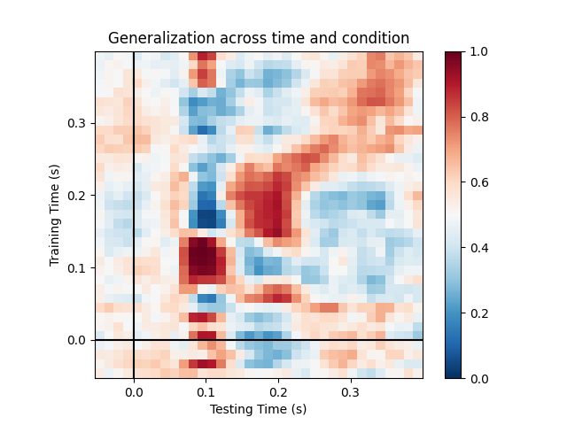
Decoding sensor space data with generalization across time and conditions#
This example runs the analysis described in [1]. It illustrates how one can fit a linear classifier to identify a discriminatory topography at a given time instant and subsequently assess whether this linear model can accurately predict all of the time samples of a second set of conditions.
# Authors: Jean-Remi King <jeanremi.king@gmail.com>
#          Alexandre Gramfort <alexandre.gramfort@inria.fr>
#          Denis Engemann <denis.engemann@gmail.com>
#
# License: BSD-3-Clause
import matplotlib.pyplot as plt

from sklearn.pipeline import make_pipeline
from sklearn.preprocessing import StandardScaler
from sklearn.linear_model import LogisticRegression

import mne
from mne.datasets import sample
from mne.decoding import GeneralizingEstimator

print(__doc__)

# Preprocess data
data_path = sample.data_path()
# Load and filter data, set up epochs
meg_path = data_path / 'MEG' / 'sample'
raw_fname = meg_path / 'sample_audvis_filt-0-40_raw.fif'
events_fname = meg_path / 'sample_audvis_filt-0-40_raw-eve.fif'
raw = mne.io.read_raw_fif(raw_fname, preload=True)
picks = mne.pick_types(raw.info, meg=True, exclude='bads')  # Pick MEG channels
raw.filter(1., 30., fir_design='firwin')  # Band pass filtering signals
events = mne.read_events(events_fname)
event_id = {'Auditory/Left': 1, 'Auditory/Right': 2,
            'Visual/Left': 3, 'Visual/Right': 4}
tmin = -0.050
tmax = 0.400
# decimate to make the example faster to run, but then use verbose='error' in
# the Epochs constructor to suppress warning about decimation causing aliasing
decim = 2
epochs = mne.Epochs(raw, events, event_id=event_id, tmin=tmin, tmax=tmax,
                    proj=True, picks=picks, baseline=None, preload=True,
                    reject=dict(mag=5e-12), decim=decim, verbose='error')
Opening raw data file /home/circleci/mne_data/MNE-sample-data/MEG/sample/sample_audvis_filt-0-40_raw.fif...
    Read a total of 4 projection items:
        PCA-v1 (1 x 10²)  idle
        PCA-v2 (1 x 10²)  idle
        PCA-v3 (1 x 10²)  idle
        Average EEG reference (1 x 60)  idle
    Range : 6450 ... 48149 =     42.956 ...   320.665 secs
Ready.
Reading 0 ... 41699  =      0.000 ...   277.709 secs...
Filtering raw data in 1 contiguous segment
Setting up band-pass filter from 1 - 30 Hz

FIR filter parameters
---------------------
Designing a one-pass, zero-phase, non-causal bandpass filter:
- Windowed time-domain design (firwin) method
- Hamming window with 0.0194 passband ripple and 53 dB stopband attenuation
- Lower passband edge: 1.00
- Lower transition bandwidth: 1.00 Hz (-6 dB cutoff frequency: 0.50 Hz)
- Upper passband edge: 30.00 Hz
- Upper transition bandwidth: 7.50 Hz (-6 dB cutoff frequency: 33.75 Hz)
- Filter length: 497 samples (3.310 sec)

[Parallel(n_jobs=1)]: Using backend SequentialBackend with 1 concurrent workers.
[Parallel(n_jobs=1)]: Done   1 out of   1 | elapsed:    0.0s remaining:    0.0s
[Parallel(n_jobs=1)]: Done   2 out of   2 | elapsed:    0.0s remaining:    0.0s
[Parallel(n_jobs=1)]: Done   3 out of   3 | elapsed:    0.0s remaining:    0.0s
[Parallel(n_jobs=1)]: Done   4 out of   4 | elapsed:    0.0s remaining:    0.0s
[Parallel(n_jobs=1)]: Done 366 out of 366 | elapsed:    0.7s finished
We will train the classifier on all left visual vs auditory trials and test on all right visual vs auditory trials.
clf = make_pipeline(
    StandardScaler(),
    LogisticRegression(solver='liblinear')  # liblinear is faster than lbfgs
)
time_gen = GeneralizingEstimator(clf, scoring='roc_auc', n_jobs=None,
                                 verbose=True)

# Fit classifiers on the epochs where the stimulus was presented to the left.
# Note that the experimental condition y indicates auditory or visual
time_gen.fit(X=epochs['Left'].get_data(),
             y=epochs['Left'].events[:, 2] > 2)
  0%|          | Fitting GeneralizingEstimator : 0/35 [00:00<?,       ?it/s]
  3%|2         | Fitting GeneralizingEstimator : 1/35 [00:00<00:01,   29.06it/s]
 11%|#1        | Fitting GeneralizingEstimator : 4/35 [00:00<00:00,   59.34it/s]
 17%|#7        | Fitting GeneralizingEstimator : 6/35 [00:00<00:00,   59.17it/s]
 23%|##2       | Fitting GeneralizingEstimator : 8/35 [00:00<00:00,   59.11it/s]
 31%|###1      | Fitting GeneralizingEstimator : 11/35 [00:00<00:00,   65.64it/s]
 40%|####      | Fitting GeneralizingEstimator : 14/35 [00:00<00:00,   69.94it/s]
 46%|####5     | Fitting GeneralizingEstimator : 16/35 [00:00<00:00,   68.17it/s]
 51%|#####1    | Fitting GeneralizingEstimator : 18/35 [00:00<00:00,   66.85it/s]
 57%|#####7    | Fitting GeneralizingEstimator : 20/35 [00:00<00:00,   65.83it/s]
 60%|######    | Fitting GeneralizingEstimator : 21/35 [00:00<00:00,   61.32it/s]
 69%|######8   | Fitting GeneralizingEstimator : 24/35 [00:00<00:00,   64.44it/s]
 74%|#######4  | Fitting GeneralizingEstimator : 26/35 [00:00<00:00,   63.87it/s]
 80%|########  | Fitting GeneralizingEstimator : 28/35 [00:00<00:00,   63.37it/s]
 89%|########8 | Fitting GeneralizingEstimator : 31/35 [00:00<00:00,   65.85it/s]
 97%|#########7| Fitting GeneralizingEstimator : 34/35 [00:00<00:00,   67.96it/s]
100%|##########| Fitting GeneralizingEstimator : 35/35 [00:00<00:00,   67.03it/s]
Score on the epochs where the stimulus was presented to the right.
scores = time_gen.score(X=epochs['Right'].get_data(),
                        y=epochs['Right'].events[:, 2] > 2)
  0%|          | Scoring GeneralizingEstimator : 0/1225 [00:00<?,       ?it/s]
  1%|1         | Scoring GeneralizingEstimator : 13/1225 [00:00<00:03,  377.84it/s]
  2%|2         | Scoring GeneralizingEstimator : 29/1225 [00:00<00:02,  425.60it/s]
  4%|3         | Scoring GeneralizingEstimator : 45/1225 [00:00<00:02,  442.00it/s]
  5%|5         | Scoring GeneralizingEstimator : 62/1225 [00:00<00:02,  458.45it/s]
  6%|6         | Scoring GeneralizingEstimator : 78/1225 [00:00<00:02,  460.90it/s]
  8%|7         | Scoring GeneralizingEstimator : 95/1225 [00:00<00:02,  468.77it/s]
  9%|9         | Scoring GeneralizingEstimator : 111/1225 [00:00<00:02,  469.25it/s]
 10%|#         | Scoring GeneralizingEstimator : 128/1225 [00:00<00:02,  474.35it/s]
 12%|#1        | Scoring GeneralizingEstimator : 144/1225 [00:00<00:02,  473.93it/s]
 13%|#3        | Scoring GeneralizingEstimator : 161/1225 [00:00<00:02,  477.18it/s]
 14%|#4        | Scoring GeneralizingEstimator : 177/1225 [00:00<00:02,  475.26it/s]
 16%|#5        | Scoring GeneralizingEstimator : 194/1225 [00:00<00:02,  478.21it/s]
 17%|#7        | Scoring GeneralizingEstimator : 211/1225 [00:00<00:02,  480.45it/s]
 18%|#8        | Scoring GeneralizingEstimator : 225/1225 [00:00<00:02,  474.00it/s]
 19%|#9        | Scoring GeneralizingEstimator : 236/1225 [00:00<00:02,  460.22it/s]
 20%|##        | Scoring GeneralizingEstimator : 247/1225 [00:00<00:02,  447.53it/s]
 22%|##1       | Scoring GeneralizingEstimator : 264/1225 [00:00<00:02,  451.73it/s]
 23%|##2       | Scoring GeneralizingEstimator : 281/1225 [00:00<00:02,  455.62it/s]
 24%|##4       | Scoring GeneralizingEstimator : 299/1225 [00:00<00:02,  461.63it/s]
 26%|##5       | Scoring GeneralizingEstimator : 314/1225 [00:00<00:01,  460.03it/s]
 27%|##6       | Scoring GeneralizingEstimator : 328/1225 [00:00<00:01,  456.50it/s]
 28%|##8       | Scoring GeneralizingEstimator : 344/1225 [00:00<00:01,  457.22it/s]
 29%|##9       | Scoring GeneralizingEstimator : 361/1225 [00:00<00:01,  460.22it/s]
 31%|###       | Scoring GeneralizingEstimator : 378/1225 [00:00<00:01,  462.66it/s]
 32%|###2      | Scoring GeneralizingEstimator : 396/1225 [00:00<00:01,  467.42it/s]
 34%|###3      | Scoring GeneralizingEstimator : 412/1225 [00:00<00:01,  467.55it/s]
 35%|###5      | Scoring GeneralizingEstimator : 429/1225 [00:00<00:01,  469.91it/s]
 36%|###6      | Scoring GeneralizingEstimator : 446/1225 [00:00<00:01,  471.89it/s]
 38%|###7      | Scoring GeneralizingEstimator : 463/1225 [00:00<00:01,  473.88it/s]
 39%|###9      | Scoring GeneralizingEstimator : 480/1225 [00:01<00:01,  475.70it/s]
 41%|####      | Scoring GeneralizingEstimator : 497/1225 [00:01<00:01,  477.36it/s]
 42%|####1     | Scoring GeneralizingEstimator : 514/1225 [00:01<00:01,  479.00it/s]
 43%|####3     | Scoring GeneralizingEstimator : 531/1225 [00:01<00:01,  480.35it/s]
 45%|####4     | Scoring GeneralizingEstimator : 549/1225 [00:01<00:01,  483.46it/s]
 46%|####6     | Scoring GeneralizingEstimator : 566/1225 [00:01<00:01,  484.58it/s]
 47%|####7     | Scoring GeneralizingEstimator : 580/1225 [00:01<00:01,  480.46it/s]
 48%|####8     | Scoring GeneralizingEstimator : 594/1225 [00:01<00:01,  476.44it/s]
 50%|####9     | Scoring GeneralizingEstimator : 609/1225 [00:01<00:01,  474.30it/s]
 51%|#####     | Scoring GeneralizingEstimator : 623/1225 [00:01<00:01,  470.54it/s]
 52%|#####2    | Scoring GeneralizingEstimator : 638/1225 [00:01<00:01,  468.95it/s]
 53%|#####3    | Scoring GeneralizingEstimator : 652/1225 [00:01<00:01,  465.74it/s]
 54%|#####4    | Scoring GeneralizingEstimator : 666/1225 [00:01<00:01,  462.74it/s]
 55%|#####5    | Scoring GeneralizingEstimator : 679/1225 [00:01<00:01,  457.90it/s]
 57%|#####6    | Scoring GeneralizingEstimator : 693/1225 [00:01<00:01,  455.39it/s]
 58%|#####8    | Scoring GeneralizingEstimator : 711/1225 [00:01<00:01,  459.61it/s]
 60%|#####9    | Scoring GeneralizingEstimator : 729/1225 [00:01<00:01,  463.66it/s]
 61%|######    | Scoring GeneralizingEstimator : 747/1225 [00:01<00:01,  467.33it/s]
 62%|######2   | Scoring GeneralizingEstimator : 765/1225 [00:01<00:00,  470.84it/s]
 64%|######3   | Scoring GeneralizingEstimator : 783/1225 [00:01<00:00,  474.24it/s]
 65%|######5   | Scoring GeneralizingEstimator : 801/1225 [00:01<00:00,  477.41it/s]
 67%|######6   | Scoring GeneralizingEstimator : 819/1225 [00:01<00:00,  479.87it/s]
 68%|######8   | Scoring GeneralizingEstimator : 838/1225 [00:01<00:00,  484.24it/s]
 70%|######9   | Scoring GeneralizingEstimator : 856/1225 [00:01<00:00,  486.55it/s]
 71%|#######1  | Scoring GeneralizingEstimator : 874/1225 [00:01<00:00,  488.93it/s]
 73%|#######2  | Scoring GeneralizingEstimator : 892/1225 [00:01<00:00,  491.18it/s]
 74%|#######4  | Scoring GeneralizingEstimator : 910/1225 [00:01<00:00,  493.24it/s]
 76%|#######5  | Scoring GeneralizingEstimator : 927/1225 [00:01<00:00,  493.65it/s]
 77%|#######7  | Scoring GeneralizingEstimator : 945/1225 [00:01<00:00,  495.39it/s]
 79%|#######8  | Scoring GeneralizingEstimator : 963/1225 [00:02<00:00,  497.21it/s]
 80%|########  | Scoring GeneralizingEstimator : 981/1225 [00:02<00:00,  498.86it/s]
 82%|########1 | Scoring GeneralizingEstimator : 999/1225 [00:02<00:00,  500.15it/s]
 83%|########3 | Scoring GeneralizingEstimator : 1018/1225 [00:02<00:00,  503.19it/s]
 85%|########4 | Scoring GeneralizingEstimator : 1036/1225 [00:02<00:00,  504.65it/s]
 86%|########5 | Scoring GeneralizingEstimator : 1053/1225 [00:02<00:00,  504.52it/s]
 87%|########6 | Scoring GeneralizingEstimator : 1064/1225 [00:02<00:00,  495.30it/s]
 88%|########7 | Scoring GeneralizingEstimator : 1075/1225 [00:02<00:00,  486.49it/s]
 89%|########9 | Scoring GeneralizingEstimator : 1091/1225 [00:02<00:00,  485.72it/s]
 91%|######### | Scoring GeneralizingEstimator : 1109/1225 [00:02<00:00,  488.04it/s]
 92%|#########2| Scoring GeneralizingEstimator : 1127/1225 [00:02<00:00,  490.18it/s]
 93%|#########3| Scoring GeneralizingEstimator : 1145/1225 [00:02<00:00,  492.29it/s]
 95%|#########5| Scoring GeneralizingEstimator : 1164/1225 [00:02<00:00,  495.89it/s]
 96%|#########6| Scoring GeneralizingEstimator : 1182/1225 [00:02<00:00,  497.75it/s]
 98%|#########7| Scoring GeneralizingEstimator : 1199/1225 [00:02<00:00,  497.98it/s]
 99%|#########9| Scoring GeneralizingEstimator : 1216/1225 [00:02<00:00,  498.13it/s]
100%|##########| Scoring GeneralizingEstimator : 1225/1225 [00:02<00:00,  492.61it/s]
100%|##########| Scoring GeneralizingEstimator : 1225/1225 [00:02<00:00,  482.35it/s]
Plot
fig, ax = plt.subplots(1)
im = ax.matshow(scores, vmin=0, vmax=1., cmap='RdBu_r', origin='lower',
                extent=epochs.times[[0, -1, 0, -1]])
ax.axhline(0., color='k')
ax.axvline(0., color='k')
ax.xaxis.set_ticks_position('bottom')
ax.set_xlabel('Testing Time (s)')
ax.set_ylabel('Training Time (s)')
ax.set_title('Generalization across time and condition')
plt.colorbar(im, ax=ax)
plt.show()
References#
Total running time of the script: ( 0 minutes 7.995 seconds)
Estimated memory usage: 128 MB