mne.time_frequency.tfr.morlet#

mne.time_frequency.tfr.morlet(sfreq, freqs, n_cycles=7.0, sigma=None, zero_mean=False)[source]#

Compute Morlet wavelets for the given frequency range.

Parameters:

sfreqfloat: The sampling Frequency.
freqsfloat | array_like, shape (n_freqs,): Frequencies to compute Morlet wavelets for.
n_cyclesfloat | array_like, shape (n_freqs,): Number of cycles. Can be a fixed number (float) or one per frequency (array-like).
sigmafloat, default None: It controls the width of the wavelet ie its temporal resolution. If sigma is None the temporal resolution is adapted with the frequency like for all wavelet transform. The higher the frequency the shorter is the wavelet. If sigma is fixed the temporal resolution is fixed like for the short time Fourier transform and the number of oscillations increases with the frequency.
zero_meanbool, default False: Make sure the wavelet has a mean of zero.

Returns:

Wslist of ndarray | ndarray: The wavelets time series. If freqs was a float, a single ndarray is returned instead of a list of ndarray.

See also

mne.time_frequency.fwhm

Notes

The Morlet wavelets follow the formulation in [1].

In wavelet analysis, the oscillation that is defined by n_cycles is tapered by a Gaussian taper, i.e., the edges of the wavelet are dampened. This means that reporting the number of cycles is not necessarily helpful for understanding the amount of temporal smoothing that has been applied (see [2]). Instead, the full width at half-maximum (FWHM) of the wavelet can be reported.

The FWHM of the wavelet at a specific frequency is defined as: \(\mathrm{FWHM} = \frac{\mathtt{n\_cycles} \times \sqrt{2 \ln{2}}}{\pi \times \mathtt{freq}}\) (cf. eq. 4 in [2]).

References

Examples

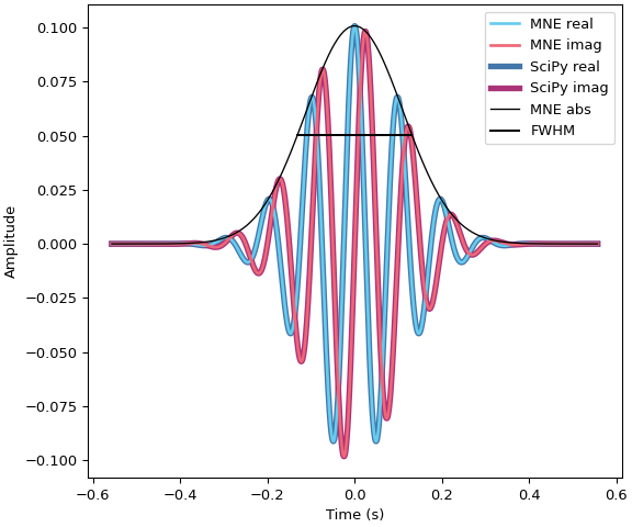
Let’s show a simple example of the relationship between n_cycles and the FWHM using mne.time_frequency.fwhm(), as well as the equivalent call using scipy.signal.morlet2():

import numpy as np
from scipy.signal import morlet2 as sp_morlet
import matplotlib.pyplot as plt
from mne.time_frequency import morlet, fwhm

sfreq, freq, n_cycles = 1000., 10, 7  # i.e., 700 ms
this_fwhm = fwhm(freq, n_cycles)
wavelet = morlet(sfreq=sfreq, freqs=freq, n_cycles=n_cycles)
M, w = len(wavelet), n_cycles # convert to SciPy convention
s = w * sfreq / (2 * freq * np.pi)  # from SciPy docs
wavelet_sp = sp_morlet(M, s, w) * np.sqrt(2)  # match our normalization

_, ax = plt.subplots(constrained_layout=True)
colors = {
    ('MNE', 'real'): '#66CCEE',
    ('SciPy', 'real'): '#4477AA',
    ('MNE', 'imag'): '#EE6677',
    ('SciPy', 'imag'): '#AA3377',
}
lw = dict(MNE=2, SciPy=4)
zorder = dict(MNE=5, SciPy=4)
t = np.arange(-M // 2 + 1, M // 2 + 1) / sfreq
for name, w in (('MNE', wavelet), ('SciPy', wavelet_sp)):
    for kind in ('real', 'imag'):
        ax.plot(t, getattr(w, kind), label=f'{name} {kind}',
                lw=lw[name], color=colors[(name, kind)],
                zorder=zorder[name])
ax.plot(t, np.abs(wavelet), label=f'MNE abs', color='k', lw=1., zorder=6)
half_max = np.max(np.abs(wavelet)) / 2.
ax.plot([-this_fwhm / 2., this_fwhm / 2.], [half_max, half_max],
        color='k', linestyle='-', label='FWHM', zorder=6)
ax.legend(loc='upper right')
ax.set(xlabel='Time (s)', ylabel='Amplitude')

../_images/mne-time_frequency-tfr-morlet-1.png