mne_connectivity.spectral_connectivity_epochs#
- mne_connectivity.spectral_connectivity_epochs(data, names=None, method='coh', indices=None, sfreq=None, *, mode='multitaper', fmin=None, fmax=inf, fdecim=1, faverage=False, tmin=None, tmax=None, mt_bandwidth=None, mt_adaptive=False, mt_low_bias=True, cwt_freqs=None, cwt_n_cycles=7, gc_n_lags=40, rank=None, n_components=1, block_size=1000, n_jobs=1, verbose=None)[source]#
Compute frequency- and time-frequency-domain connectivity measures.
The connectivity method(s) are specified using the “method” parameter. All methods are based on estimates of the cross- and power spectral densities (CSD/PSD) Sxy and Sxx, Syy.
- Parameters:
- dataarray_like, shape (n_epochs, n_signals, n_times) |
Epochs| generator |EpochsSpectrum|EpochsTFR The data from which to compute connectivity. Can be epoched time series data as an array-like or
mne.Epochsobject, or Fourier coefficients for each epoch as anmne.time_frequency.EpochsSpectrumormne.time_frequency.EpochsTFRobject. If time series data, the spectral information will be computed according to the spectral estimation mode (see themodeparameter). If anmne.time_frequency.EpochsSpectrumormne.time_frequency.EpochsTFRobject, existing spectral information will be used and themodeparameter will be ignored.Note that it is also possible to combine multiple time series signals by providing a list of tuples, e.g.:
data = [(arr_0, stc_0), (arr_1, stc_1), (arr_2, stc_2)]
which corresponds to 3 epochs where
arr_*is an array with the same number of time points asstc_*. Data can also be a list/generator of arrays, shape(n_signals, n_times), or a list/generator ofmne.SourceEstimateormne.VolSourceEstimateobjects.Changed in version 0.8: Fourier coefficients stored in an
mne.time_frequency.EpochsSpectrumormne.time_frequency.EpochsTFRobject can also be passed in as data. Storing Fourier coefficients inmne.time_frequency.EpochsSpectrumobjects requiresmne >= 1.8. Storing multitaper weights inmne.time_frequency.EpochsTFRobjects requiresmne >= 1.10.- namesarray_like |
None The names of the nodes of the dataset used to compute connectivity. If
None(default), then names will be a list of integers from 0 ton_nodes. If a list of names, then it must be equal in length ton_nodes.- method
str|listofstr Connectivity measure(s) to compute. These can be
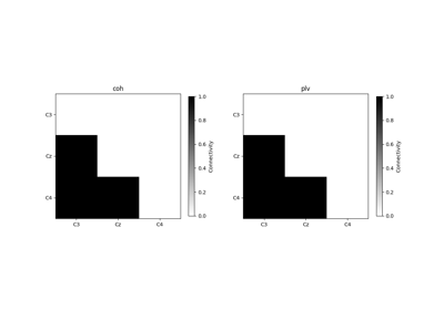
['coh', 'cohy', 'imcoh',
'cacoh', 'mic', 'mim', 'plv', 'ciplv', 'ppc', 'pli', 'dpli', 'wpli',
'wpli2_debiased', 'gc', 'gc_tr']
. These are:‘coh’ : Coherence
‘cohy’ : Coherency
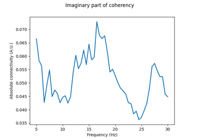
‘imcoh’ : Imaginary part of Coherency
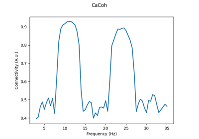
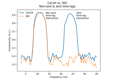
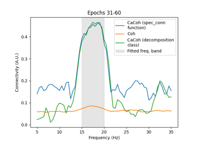
‘cacoh’ : Canonical Coherency (CaCoh)
‘mic’ : Maximised Imaginary part of Coherency (MIC)
‘mim’ : Multivariate Interaction Measure (MIM)
‘plv’ : Phase-Locking Value (PLV)
‘ciplv’ : Corrected Imaginary PLV (ciPLV)
‘ppc’ : Pairwise Phase Consistency (PPC)
‘pli’ : Phase Lag Index (PLI)
‘pli2_unbiased’ : Unbiased estimator of squared PLI
‘dpli’ : Directed PLI (DPLI)
‘wpli’ : Weighted PLI (WPLI)
‘wpli2_debiased’ : Debiased estimator of squared WPLI
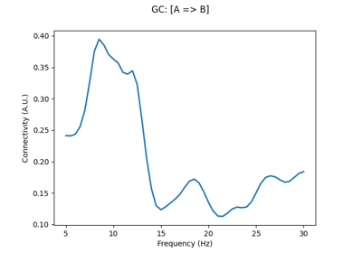
‘gc’ : State-space Granger Causality (GC)
‘gc_tr’ : State-space GC on time-reversed signals
Multivariate methods (
['cacoh', 'mic', 'mim', 'gc', 'gc_tr']) cannot be called with the other methods.- indices
tupleof array_like |None Two array-likes with indices of connections for which to compute connectivity. If a bivariate method is called, each array for the seeds and targets should contain the channel indices for each bivariate connection. If a multivariate method is called, each array for the seeds and targets should consist of nested arrays containing the channel indices for each multivariate connection. If
None, connections between all channels are computed, unless a Granger causality method is called, in which case an error is raised.- sfreq
float|None The sampling frequency. Required if
datais an array-like.- mode
'multitaper'|'fourier'|'cwt_morlet' Spectrum estimation mode. Ignored if
datais anmne.time_frequency.EpochsSpectrumormne.time_frequency.EpochsTFRobject.- fmin
float|tupleoffloat|None The lower frequency of interest. Multiple bands are defined using a tuple, e.g., (8., 20.) for two bands with 8 Hz and 20 Hz lower freq. If
None, the frequency corresponding to 5 cycles based on the epoch length is used. For example, with an epoch length of 1 sec, the lower frequency would be 5 / 1 sec = 5 Hz.- fmax
float|tupleoffloat The upper frequency of interest. Multiple bands are defined using a tuple, e.g., (13., 30.) for two bands with 13 Hz and 30 Hz upper freq.
- fdecim
int|None Decimation factor in the frequency domain. Selects every Nth frequency bin from the (time-)frequency decomposition (where N is the value of
fdecim). If 1 (default), no decimation occurs.Added in version 0.8.
- faveragebool
Average connectivity scores for each frequency band. If
True, the output freqs will be a list with arrays of the frequencies that were averaged.- tmin
float|None Time to start connectivity estimation. Note: when
datais an array-like, the first sample is assumed to be at time 0. Formne.Epochs, the time information contained in the object is used to compute the time indices. Ignored ifdatais anmne.time_frequency.EpochsSpectrumobject.- tmax
float|None Time to end connectivity estimation. Note: when
datais an array-like, the first sample is assumed to be at time 0. Formne.Epochs, the time information contained in the object is used to compute the time indices. Ignored ifdatais anmne.time_frequency.EpochsSpectrumobject.- mt_bandwidth
float|None The bandwidth of the multitaper windowing function in Hz. Only used in
'multitaper'mode. Ignored ifdatais anmne.time_frequency.EpochsSpectrumormne.time_frequency.EpochsTFRobject.- mt_adaptivebool
Use adaptive weights to combine the tapered spectra into PSD. Only used in
'multitaper'mode. Ignored ifdatais anmne.time_frequency.EpochsSpectrumormne.time_frequency.EpochsTFRobject.- mt_low_biasbool
Only use tapers with more than 90 percent spectral concentration within bandwidth. Only used in
'multitaper'mode. Ignored ifdatais anmne.time_frequency.EpochsSpectrumormne.time_frequency.EpochsTFRobject.- cwt_freqsarray_like
Array-like of frequencies of interest. Only used in
'cwt_morlet'mode. Only the frequencies within the range specified byfminandfmaxare used. Ignored ifdatais anmne.time_frequency.EpochsSpectrumormne.time_frequency.EpochsTFRobject.- cwt_n_cycles
float| array_like Number of cycles. Fixed number or one per frequency. Only used in
'cwt_morlet'mode. Ignored ifdatais anmne.time_frequency.EpochsSpectrumormne.time_frequency.EpochsTFRobject.- gc_n_lags
int Number of lags to use for the vector autoregressive model when computing Granger causality. Higher values increase computational cost, but reduce the degree of spectral smoothing in the results. Only used if
methodcontains any of['gc', 'gc_tr'].- rank
tupleof array_like |None Two array-likes with the rank to project the seed and target data to, respectively, using singular value decomposition. If
None, the rank of the data is computed and projected to. Only used ifmethodcontains any of['cacoh', 'mic', 'mim', 'gc', 'gc_tr'].- n_components
int|None Number of connectivity components to extract from the data. If an int, the number of components must be <= the minimum rank of the seeds and targets. E.g., if the seed channels had a rank of 5 and the target channels had a rank of 3,
n_componentsmust be <= 3. IfNone, the number of components equal to the minimum rank of the seeds and targets is extracted (see therankparameter). Only used ifmethodcontains any of['cacoh', 'mic'].Added in version 0.8.
- block_size
int How many connections to compute at once (higher numbers are faster but require more memory).
- n_jobs
int How many samples to process in parallel.
- verbosebool |
str|int|None If not
None, override default verbose level (seemne.verbose()for more info). If used, it should be passed as a keyword-argument only.
- dataarray_like, shape (n_epochs, n_signals, n_times) |
- Returns:
- coninstance of
SpectralConnectivityorSpectroTemporalConnectivity|list Computed connectivity measure(s). An instance of
SpectralConnectivity,SpectroTemporalConnectivity, or a list of instances corresponding to connectivity measures if several connectivity measures are specified. The shape of the connectivity result will be:(n_cons, n_freqs)for'multitaper'or'fourier'modes(n_cons, n_freqs, n_times)for'cwt_morlet'mode(n_cons, n_comps, n_freqs[, n_times])for valid multivariate methods ifn_components > 1n_cons = n_signals ** 2for bivariate methods withindices=Nonen_cons = 1for multivariate methods withindices=Nonen_cons = len(indices[0])for bivariate and multivariate methods whenindicesis supplied
- coninstance of
See also
Notes
Please note that the interpretation of the measures in this function depends on the data and underlying assumptions and does not necessarily reflect a causal relationship between brain regions.
These measures are not to be interpreted over time. Each epoch passed into the dataset is interpreted as an independent sample of the same connectivity structure. Within each epoch, it is assumed that the spectral measure is stationary. The spectral measures implemented in this function are computed across epochs. Thus, spectral measures computed with only one epoch will result in errorful values and spectral measures computed with few Epochs will be unreliable. Please see
spectral_connectivity_time()for time-resolved connectivity estimation.The spectral densities can be estimated using a multitaper method with digital prolate spheroidal sequence (DPSS) windows, a discrete Fourier transform with Hanning windows, or a continuous wavelet transform using Morlet wavelets. The spectral estimation mode is specified using the
modeparameter. Complex Welch, multitaper, or Morlet coefficients can also be passed in as data in the form ofmne.time_frequency.EpochsSpectrumormne.time_frequency.EpochsTFRobjects.By default, the connectivity between all signals is computed (only connections corresponding to the lower-triangular part of the connectivity matrix). If one is only interested in the connectivity between some signals, the
indicesparameter can be used. For example, to compute the connectivity between the signal with index 0 and signals “2, 3, 4” (a total of 3 connections) one can use the following:indices = (np.array([0, 0, 0]), # row indices np.array([2, 3, 4])) # col indices con = spectral_connectivity_epochs(data, method='coh', indices=indices, ...)
In this case
con.get_data().shape = (3, n_freqs). The connectivity scores are in the same order as defined indices.For multivariate methods, this is handled differently. If
indicesisNone, connectivity between all signals will be computed and a single connectivity spectrum will be returned (this is not possible if a Granger causality method is called). Ifindicesis specified, seed and target indices for each connection should be specified as nested array-likes. For example, to compute the connectivity between signals (0, 1) -> (2, 3) and (0, 1) -> (4, 5), indices should be specified as:indices = (np.array([[0, 1], [0, 1]]), # seeds np.array([[2, 3], [4, 5]])) # targets
More information on working with multivariate indices and handling connections where the number of seeds and targets are not equal can be found in the Working with ragged indices for multivariate connectivity example.
Supported Connectivity Measures
The connectivity method(s) is specified using the
methodparameter. The following methods are supported (note:E[]denotes average over epochs). Multiple measures can be computed at once by using a list/tuple, e.g.,['coh', 'pli']to compute coherence and PLI.‘coh’ : Coherence given by:
         | E[Sxy] |
C = ---------------------
    sqrt(E[Sxx] * E[Syy])
‘cohy’ : Coherency given by:
           E[Sxy]
C = ---------------------
    sqrt(E[Sxx] * E[Syy])
‘imcoh’ : Imaginary coherence [1] given by:
          Im(E[Sxy])
C = ----------------------
    sqrt(E[Sxx] * E[Syy])
‘cacoh’ : Canonical Coherency (CaCoh) [2] given by:
\(\textrm{CaCoh}=\Large{\frac{\boldsymbol{a}^T\boldsymbol{D} (\Phi)\boldsymbol{b}}{\sqrt{\boldsymbol{a}^T\boldsymbol{a} \boldsymbol{b}^T\boldsymbol{b}}}}\)
where: \(\boldsymbol{D}(\Phi)\) is the cross-spectral density between seeds and targets transformed for a given phase angle \(\Phi\); and \(\boldsymbol{a}\) and \(\boldsymbol{b}\) are eigenvectors for the seeds and targets, such that \(\boldsymbol{a}^T\boldsymbol{D}(\Phi) \boldsymbol{b}\) maximises coherency between the seeds and targets. Taking the absolute value of the results gives maximised coherence.
‘mic’ : Maximised Imaginary part of Coherency (MIC) [3] given by:
\(\textrm{MIC}=\Large{\frac{\boldsymbol{\alpha}^T \boldsymbol{E \beta}}{\parallel\boldsymbol{\alpha}\parallel \parallel\boldsymbol{\beta}\parallel}}\)
where: \(\boldsymbol{E}\) is the imaginary part of the transformed cross-spectral density between seeds and targets; and \(\boldsymbol{\alpha}\) and \(\boldsymbol{\beta}\) are eigenvectors for the seeds and targets, such that \(\boldsymbol{\alpha}^T \boldsymbol{E \beta}\) maximises the imaginary part of coherency between the seeds and targets.
‘mim’ : Multivariate Interaction Measure (MIM) [3] given by:
\(\textrm{MIM}=tr(\boldsymbol{EE}^T)\)
where \(\boldsymbol{E}\) is the imaginary part of the transformed cross-spectral density between seeds and targets.
‘plv’ : Phase-Locking Value (PLV) [4] given by:
PLV = |E[Sxy/|Sxy|]|
‘ciplv’ : corrected imaginary PLV (ciPLV) [5] given by:
                 |E[Im(Sxy/|Sxy|)]|
ciPLV = ------------------------------------
         sqrt(1 - |E[real(Sxy/|Sxy|)]| ** 2)
‘ppc’ : Pairwise Phase Consistency (PPC), an unbiased estimator of squared PLV [6].
‘pli’ : Phase Lag Index (PLI) [7] given by:
PLI = |E[sign(Im(Sxy))]|
‘pli2_unbiased’ : Unbiased estimator of squared PLI [8].
‘dpli’ : Directed Phase Lag Index (DPLI) [9] given by (where H is the Heaviside function):
DPLI = E[H(Im(Sxy))]
‘wpli’ : Weighted Phase Lag Index (WPLI) [8] given by:
          |E[Im(Sxy)]|
WPLI = ------------------
          E[|Im(Sxy)|]
‘wpli2_debiased’ : Debiased estimator of squared WPLI [8].
‘gc’ : State-space Granger Causality (GC) [10] given by:
\(GC = ln\Large{(\frac{\lvert\boldsymbol{S}_{tt}\rvert}{\lvert \boldsymbol{S}_{tt}-\boldsymbol{H}_{ts}\boldsymbol{\Sigma}_{ss \lvert t}\boldsymbol{H}_{ts}^*\rvert}})\)
where: \(s\) and \(t\) represent the seeds and targets, respectively; \(\boldsymbol{H}\) is the spectral transfer function; \(\boldsymbol{\Sigma}\) is the residuals matrix of the autoregressive model; and \(\boldsymbol{S}\) is \(\boldsymbol{\Sigma}\) transformed by \(\boldsymbol{H}\).
‘gc_tr’ : State-space GC on time-reversed signals [10][11] given by the same equation as for
'gc', but where the autocovariance sequence from which the autoregressive model is produced is transposed to mimic the reversal of the original signal in time [12].References
Examples using mne_connectivity.spectral_connectivity_epochs#
Comparing spectral connectivity computed over time or over trials

Compute seed-based time-frequency connectivity in sensor space
Multivariate decomposition for efficient connectivity analysis
Compute directionality of connectivity with multivariate Granger causality

Working with ragged indices for multivariate connectivity
Compute multivariate measures of the imaginary part of coherency
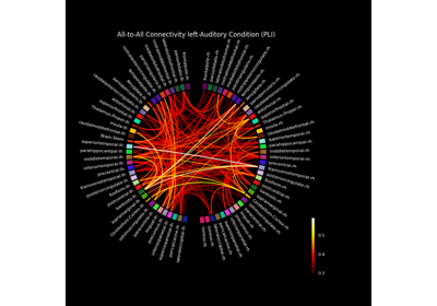
Compute mixed source space connectivity and visualize it using a circular graph
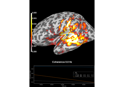
Compute coherence in source space using a MNE inverse solution
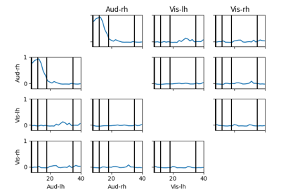
Compute full spectrum source space connectivity between labels
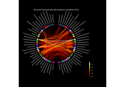
Compute source space connectivity and visualize it using a circular graph
Determine the significance of connectivity estimates against baseline connectivity