mne_connectivity.spectral_connectivity_time

mne_connectivity.spectral_connectivity_time(data, freqs=None, method='coh', average=False, indices='lower', sfreq=None, *, fmin=None, fmax=None, fdecim=1, faverage=False, sm_times=0.0, sm_freqs=1, sm_kernel='hanning', padding=0.0, mode='cwt_morlet', mt_bandwidth=None, n_cycles=7.0, gc_n_lags=40, rank=None, n_components=1, decim=1, n_jobs=1, verbose=None)

Compute time-frequency-domain connectivity measures.

This function computes spectral connectivity over time from epoched data. The data may consist of a single epoch.

The connectivity method(s) are specified using the method parameter. All methods are based on time-resolved estimates of the cross- and power spectral densities (CSD/PSD) Sxy and Sxx, Syy.

Parameters:

dataarray_like, shape (n_epochs, n_signals, n_times) | Epochs | EpochsTFR

The data from which to compute connectivity. Can be epoched time series data as an array-like or mne.Epochs object, or Fourier coefficients for each epoch as an mne.time_frequency.EpochsTFR object. If time series data, the spectral information will be computed according to the spectral estimation mode (see the mode parameter). If an mne.time_frequency.EpochsTFR object, existing spectral information will be used and the mode parameter will be ignored.

Changed in version 0.8: Fourier coefficients stored in an mne.time_frequency.EpochsTFR object can also be passed in as data. Storing multitaper weights in mne.time_frequency.EpochsTFR objects requires mne >= 1.10.

freqsarray_like | None

Array-like of frequencies of interest for time-frequency decomposition. Only the frequencies within the range specified by fmin and fmax are used. If data is an array-like or mne.Epochs object, the frequencies must be specified. If data is an mne.time_frequency.EpochsTFR object, data.freqs is used and this parameter is ignored.

methodstr | list of str

Connectivity measure(s) to compute. These can be ['coh', 'cohy', 'imcoh', 'cacoh', 'mic', 'mim', 'plv', 'ciplv', 'pli', 'wpli', 'gc', 'gc_tr']. These are:

• ‘coh’ : Coherence

• ‘cohy’ : Coherency

• ‘imcoh’ : Imaginary part of Coherency

• ‘cacoh’ : Canonical Coherency (CaCoh)

• ‘mic’ : Maximised Imaginary part of Coherency (MIC)

• ‘mim’ : Multivariate Interaction Measure (MIM)

• ‘plv’ : Phase-Locking Value (PLV)

• ‘ciplv’ : Corrected Imaginary PLV (ciPLV)

• ‘pli’ : Phase Lag Index (PLI)

• ‘wpli’ : Weighted PLI (WPLI)

• ‘gc’ : State-space Granger Causality (GC)

• ‘gc_tr’ : State-space GC on time-reversed signals

Multivariate methods (['cacoh', 'mic', 'mim', 'gc', 'gc_tr']) cannot be called with the other methods.

averagebool

Average connectivity scores over epochs. If True, output will be an instance of SpectralConnectivity, otherwise EpochSpectralConnectivity.

indicestuple of array_like | 'lower' | 'upper' | 'all'

The indices of channels to compute connectivity between. If a tuple, then must contain two array-likes, where the first array represents the channel indices of the seeds, and the second array represents the channel indices of the targets. For multivariate methods, the seed and target indices should consist of nested arrays containing the channel indices for each multivariate connection. See the notes section for more information. If 'lower', compute the lower-triangular part of the connectivity matrix. If 'upper', compute the upper-triangular part of the connectivity matrix. If 'all', compute all connections. Default is 'lower'.

sfreqfloat | None

The sampling frequency. Required if data is not an mne.Epochs or mne.time_frequency.EpochsTFR object.

fminfloat | tuple of float | None

The lower frequency of interest. Multiple bands are defined using a tuple, e.g., (8., 20.) for two bands with 8 Hz and 20 Hz lower bounds. If None, the lowest frequency in freqs is used.

fmaxfloat | tuple of float | None

The upper frequency of interest. Multiple bands are defined using a tuple, e.g. (13., 30.) for two band with 13 Hz and 30 Hz upper bounds. If None, the highest frequency in freqs is used.

fdecimint | None

Decimation factor in the frequency domain. Selects every Nth frequency bin from the (time-)frequency decomposition (where N is the value of fdecim). If 1 (default), no decimation occurs.

Added in version 0.8.

faveragebool

Average connectivity scores for each frequency band. If True, the output freqs will be an array of the average frequencies of each band.

sm_timesfloat

Amount of time to consider for the temporal smoothing in seconds. If 0, no temporal smoothing is applied.

sm_freqsint

Number of points for frequency smoothing. By default, 1 is used which is equivalent to no smoothing.

sm_kernel'square' | 'hanning'

Smoothing kernel type. For 'hanning', see numpy.hanning().

paddingfloat

Amount of time to consider as padding at the beginning and end of each epoch in seconds. See Notes for more information.

mode'multitaper' | 'cwt_morlet'

Time-frequency decomposition method. See mne.time_frequency.tfr_array_multitaper() and mne.time_frequency.tfr_array_morlet() for reference. Ignored if data is an mne.time_frequency.EpochsTFR object.

mt_bandwidthfloat | None

Product between the temporal window length (in seconds) and the full frequency bandwidth (in Hz). This product can be seen as the surface of the window on the time/frequency plane and controls the frequency bandwidth (thus the frequency resolution) and the number of good tapers. See mne.time_frequency.tfr_array_multitaper() documentation. Ignored if data is an mne.time_frequency.EpochsTFR object.

n_cyclesfloat | array_like

Number of cycles in the wavelet, either a fixed number or one per frequency. The number of cycles n_cycles and the frequencies of interest freqs define the temporal window length. For details, see mne.time_frequency.tfr_array_multitaper() and mne.time_frequency.tfr_array_morlet() documentation. Ignored if data is an mne.time_frequency.EpochsTFR object.

gc_n_lagsint

Number of lags to use for the vector autoregressive model when computing Granger causality. Higher values increase computational cost, but reduce the degree of spectral smoothing in the results. Only used if method contains any of ['gc', 'gc_tr'].

ranktuple of array_like | None

Two array-likes with the rank to project the seed and target data to, respectively, using singular value decomposition. If None, the rank of the data is computed and projected to. Only used if method contains any of ['cacoh', 'mic', 'mim', 'gc', 'gc_tr'].

n_componentsint | None

Number of connectivity components to extract from the data. If an int, the number of components must be <= the minimum rank of the seeds and targets. E.g., if the seed channels had a rank of 5 and the target channels had a rank of 3, n_components must be <= 3. If None, the number of components equal to the minimum rank of the seeds and targets is extracted (see the rank parameter). Only used if method contains any of ['cacoh', 'mic'].

Added in version 0.8.

decimint

Decimation factor in the time domain. Selects every Nth time bin from the time-frequency decomposition (where N is the value of decim). If 1 (default), no decimation occurs.

n_jobsint

Number of connections to compute in parallel. Memory mapping must be activated. Please see the Notes section for details.

verbosebool | str | int | None

If not None, override default verbose level (see mne.verbose() for more info). If used, it should be passed as a keyword-argument only.

Returns:

coninstance of EpochSpectralConnectivity or SpectralConnectivity | list

Computed connectivity measure(s). An instance of EpochSpectralConnectivity, SpectralConnectivity, or a list of instances corresponding to connectivity measures if several connectivity measures are specified. The shape of each connectivity dataset is ([n_epochs,] n_cons, [n_comps,] n_freqs):

• n_comps is present for valid multivariate methods if n_components > 1

• When indices is 'all', n_cons = n_signals ** 2

• When indices is 'lower' or 'upper', n_cons = n_signals * (n_signals - 1) / 2

• When indices is a tuple of array-likes, n_cons = len(indices[0])

See also

mne_connectivity.spectral_connectivity_epochs

mne_connectivity.SpectralConnectivity

mne_connectivity.EpochSpectralConnectivity

Notes

Please note that the interpretation of the measures in this function depends on the data and underlying assumptions and does not necessarily reflect a causal relationship between brain regions.

The connectivity measures are computed over time within each epoch and optionally averaged over epochs. High connectivity values indicate that the phase coupling (interpreted as estimated connectivity) differences between signals stay consistent over time.

The spectral densities can be estimated using a multitaper method with digital prolate spheroidal sequence (DPSS) windows, or a continuous wavelet transform using Morlet wavelets. The spectral estimation mode is specified using the mode parameter.

When using the multitaper spectral estimation method, the cross-spectral density is computed separately for each taper and aggregated using a weighted average, where the weights correspond to the concentration ratios between the DPSS windows.

Spectral estimation using multitaper or Morlet wavelets introduces edge effects that depend on the length of the wavelet. To remove edge effects, the parameter padding can be used to prune the edges of the signal. Please see the documentation of mne.time_frequency.tfr_array_multitaper() and mne.time_frequency.tfr_array_morlet() for details on wavelet length (i.e., time window length).

Complex multitaper, or Morlet coefficients can also be passed in as data in the form of mne.time_frequency.EpochsTFR objects.

If connectivity for all possible connections is desired, we can save time and memory by only computing and storing the lower- (or upper-) triangular part of the connectivity matrix. When the full set of connectivity values is needed, the missing values can be inferred based on what has been computed. See the notes section of the get_data() method in the connectivity containers for more information.

If one is only interested in the connectivity between some signals, the indices parameter can be specified as a tuple of array-likes. For example, to compute the connectivity between the signal with index 0 and the signals with indices 2, 3, and 4 (a total of 3 connections) one can use the following:

indices = (np.array([0, 0, 0]),  # seed indices
           np.array([2, 3, 4]))  # target indices

For multivariate methods, indices must be specified as a tuple, where the seed and target indices for each connection are nested array-likes. For example, to compute the connectivity between signals (0, 1) → (2, 3) and (0, 1) → (4, 5), indices should be specified as:

indices = (np.array([[0, 1], [0, 1]]),  # seeds
           np.array([[2, 3], [4, 5]]))  # targets

More information on working with multivariate indices and handling connections where the number of seeds and targets are not equal can be found in the Working with ragged indices for multivariate connectivity example.

Supported Connectivity Measures

The connectivity method(s) is specified using the method parameter. The following methods are supported (note: E[] denotes average over epochs). Multiple measures can be computed at once by using a list/tuple, e.g., ['coh', 'pli'] to compute coherence and PLI.

‘coh’ : Coherence given by:

         | E[Sxy] |
C = ---------------------
    sqrt(E[Sxx] * E[Syy])

‘cohy’ : Coherency given by:

           E[Sxy]
C = ---------------------
    sqrt(E[Sxx] * E[Syy])

‘imcoh’ : Imaginary coherence [1] given by:

          Im(E[Sxy])
C = ----------------------
    sqrt(E[Sxx] * E[Syy])

‘cacoh’ : Canonical Coherency (CaCoh) [2] given by:

\(\textrm{CaCoh}=\Large{\frac{\boldsymbol{a}^T\boldsymbol{D} (\Phi)\boldsymbol{b}}{\sqrt{\boldsymbol{a}^T\boldsymbol{a} \boldsymbol{b}^T\boldsymbol{b}}}}\)

where: \(\boldsymbol{D}(\Phi)\) is the cross-spectral density between seeds and targets transformed for a given phase angle \(\Phi\); and \(\boldsymbol{a}\) and \(\boldsymbol{b}\) are eigenvectors for the seeds and targets, such that \(\boldsymbol{a}^T\boldsymbol{D}(\Phi) \boldsymbol{b}\) maximises coherency between the seeds and targets. Taking the absolute value of the results gives maximised coherence.

‘mic’ : Maximised Imaginary part of Coherency (MIC) [3] given by:

\(\textrm{MIC}=\Large{\frac{\boldsymbol{\alpha}^T \boldsymbol{E \beta}}{\parallel\boldsymbol{\alpha}\parallel \parallel\boldsymbol{\beta}\parallel}}\)

where: \(\boldsymbol{E}\) is the imaginary part of the transformed cross-spectral density between seeds and targets; and \(\boldsymbol{\alpha}\) and \(\boldsymbol{\beta}\) are eigenvectors for the seeds and targets, such that \(\boldsymbol{\alpha}^T \boldsymbol{E \beta}\) maximises the imaginary part of coherency between the seeds and targets.

‘mim’ : Multivariate Interaction Measure (MIM) [3] given by:

\(\textrm{MIM}=tr(\boldsymbol{EE}^T)\)

where \(\boldsymbol{E}\) is the imaginary part of the transformed cross-spectral density between seeds and targets.

‘plv’ : Phase-Locking Value (PLV) [4] given by:

PLV = |E[Sxy/|Sxy|]|

‘ciplv’ : Corrected imaginary PLV (ciPLV) [5] given by:

                 |E[Im(Sxy/|Sxy|)]|
ciPLV = ------------------------------------
         sqrt(1 - |E[real(Sxy/|Sxy|)]| ** 2)

‘pli’ : Phase Lag Index (PLI) [6] given by:

PLI = |E[sign(Im(Sxy))]|

‘wpli’ : Weighted Phase Lag Index (WPLI) [7] given by:

          |E[Im(Sxy)]|
WPLI = ------------------
          E[|Im(Sxy)|]

‘gc’ : State-space Granger Causality (GC) [8] given by:

\(GC = ln\Large{(\frac{\lvert\boldsymbol{S}_{tt}\rvert}{\lvert \boldsymbol{S}_{tt}-\boldsymbol{H}_{ts}\boldsymbol{\Sigma}_{ss \lvert t}\boldsymbol{H}_{ts}^*\rvert}})\)

where: \(s\) and \(t\) represent the seeds and targets, respectively; \(\boldsymbol{H}\) is the spectral transfer function; \(\boldsymbol{\Sigma}\) is the residuals matrix of the autoregressive model; and \(\boldsymbol{S}\) is \(\boldsymbol{\Sigma}\) transformed by \(\boldsymbol{H}\).

‘gc_tr’ : State-space GC on time-reversed signals [8][9] given by the same equation as for 'gc', but where the autocovariance sequence from which the autoregressive model is produced is transposed to mimic the reversal of the original signal in time [10].

Parallel computation can be activated by setting the n_jobs parameter. Under the hood, this utilizes the joblib library. For effective parallelization, you should activate memory mapping in MNE-Python by setting MNE_MEMMAP_MIN_SIZE and MNE_CACHE_DIR. Activating memory mapping will make joblib store arrays greater than the minimum size on disc, and forego direct RAM access for more efficient processing. For example, in your code, run:

mne.set_config('MNE_MEMMAP_MIN_SIZE', '10M')
mne.set_config('MNE_CACHE_DIR', '/dev/shm')

When MNE_MEMMAP_MIN_SIZE=None, the underlying joblib implementation results in pickling and unpickling the whole array each time a pair of indices is accessed, which is slow, compared to memory mapping the array.

This function is based on the frites.conn.conn_spec implementation in Frites.

Added in version 0.3.

References

[1]

Guido Nolte, Ou Bai, Lewis Wheaton, Zoltan Mari, Sherry Vorbach, and Mark Hallett. Identifying true brain interaction from EEG data using the imaginary part of coherency. Clinical Neurophysiology, 115(10):2292–2307, 2004. doi:10.1016/j.clinph.2004.04.029.

[2]

Carmen Vidaurre, Guido Nolte, Ingmar E.J. de Vries, M. Gómez, Tjeerd W. Boonstra, K.-R. Müller, Arno Villringer, and Vadim V. Nikulin. Canonical maximization of coherence: a novel tool for investigation of neuronal interactions between two datasets. NeuroImage, 201:116009, 2019. doi:10.1016/j.neuroimage.2019.116009.

[3] (1,2)

Arne Ewald, Laura Marzetti, Filippo Zappasodi, Frank C. Meinecke, and Guido Nolte. Estimating true brain connectivity from EEG/MEG data invariant to linear and static transformations in sensor space. NeuroImage, 60(1):476–488, 2012. doi:10.1016/j.neuroimage.2011.11.084.

[4]

Jean-Philippe Lachaux, Eugenio Rodriguez, Jacques Martinerie, and Francisco J. Varela. Measuring phase synchrony in brain signals. Human Brain Mapping, 8(4):194–208, 1999. doi:10.1002/(SICI)1097-0193(1999)8:4<194::AID-HBM4>3.0.CO;2-C.

[5]

Ernesto Pereda Ricardo Bruña, Fernando Maestú. Phase locking value revisited: teaching new tricks to an old dog. Journal of Neural Engineering, 15(5):056011, 2018. doi:10.1088/1741-2552/aacfe4.

[6]

Cornelis J. Stam, Guido Nolte, and Andreas Daffertshofer. Phase lag index: assessment of functional connectivity from multi channel EEG and MEG with diminished bias from common sources. Human Brain Mapping, 28(11):1178–1193, 2007. doi:10.1002/hbm.20346.

[7]

Martin Vinck, Robert Oostenveld, Marijn van Wingerden, Franscesco Battaglia, and Cyriel M.A. Pennartz. An improved index of phase-synchronization for electrophysiological data in the presence of volume-conduction, noise and sample-size bias. NeuroImage, 55(4):1548–1565, 2011. doi:10.1016/j.neuroimage.2011.01.055.

[8] (1,2)

Lionel Barnett and Anil K. Seth. Granger causality for state-space models. Physical Review E, 91(4):040101, 2015. doi:10.1103/PhysRevE.91.040101.

[9]

Irene Winkler, Danny Panknin, Daniel Bartz, Klaus-Robert Müller, and Stefan Haufe. Validity of time reversal for testing granger causality. IEEE Transactions on Signal Processing, 64(11):2746–2760, 2016. doi:10.1109/TSP.2016.2531628.

[10]

Stefan Haufe, Vadim V Nikulin, and Guido Nolte. Alleviating the influence of weak data asymmetries on granger-causal analyses. In Latent Variable Analysis and Signal Separation: 10th International Conference, LVA/ICA 2012, Tel Aviv, Israel, March 12-15, 2012. Proceedings 10, 25–33. Springer, 2012. doi:10.1007/978-3-642-28551-6_4.

Examples using mne_connectivity.spectral_connectivity_time

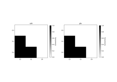
Comparing spectral connectivity computed over time or over trials

Comparing spectral connectivity computed over time or over trials

Multivariate decomposition for efficient connectivity analysis

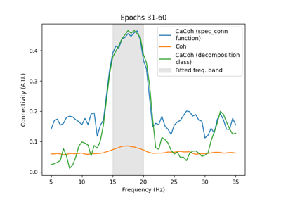
Multivariate decomposition for efficient connectivity analysis