Note
Go to the end to download the full example code.
Bandpower rolling window🔗
With a StreamLSL, we can compute the bandpower on a time
rolling window. For this example, we will look at the alpha band power, between 8 and
13 Hz.
import time
import uuid

import numpy as np
from matplotlib import colormaps
from matplotlib import pyplot as plt
from mne.io import read_raw_fif
from mne.time_frequency import psd_array_multitaper
from numpy.typing import NDArray
from scipy.integrate import simpson
from scipy.signal import periodogram, welch

from mne_lsl.datasets import sample
from mne_lsl.player import PlayerLSL
from mne_lsl.stream import StreamLSL

# dataset used in the example
raw = read_raw_fif(sample.data_path() / "sample-ant-raw.fif", preload=False)
raw.crop(40, 60).load_data()
raw
Preprocessing🔗
In a real-time scenario, we would want to apply artifact rejection methods online to estimate the bandpower on brain signals, not on artifacts. For this example, we will only apply a bandpass filter to the data.
Estimating the bandpower🔗
First, we will define the function estimating the bandpower on a time window. The
bandpower will be estimated by integrating the power spectral density (PSD) on the
frequency band of interest, using the composite Simpson’s rule
(scipy.integrate.simpson()).
def bandpower(
    data: NDArray[np.float64],
    fs: float,
    method: str,
    band: tuple[float, float],
    relative: bool = True,
    **kwargs,
) -> NDArray[np.float64]:
    """Compute the bandpower of the individual channels.

    Parameters
    ----------
    data : array of shape (n_channels, n_samples)
        Data on which the the bandpower is estimated.
    fs : float
        Sampling frequency in Hz.
    method : 'periodogram' | 'welch' | 'multitaper'
        Method used to estimate the power spectral density.
    band : tuple of shape (2,)
        Frequency band of interest in Hz as 2 floats, e.g. ``(8, 13)``. The
        edges are included.
    relative : bool
        If True, the relative bandpower is returned instead of the absolute
        bandpower.
    **kwargs : dict
        Additional keyword arguments are provided to the power spectral density
        estimation function.
        * 'periodogram': scipy.signal.periodogram
        * 'welch'``: scipy.signal.welch
        * 'multitaper': mne.time_frequency.psd_array_multitaper

        The only provided arguments are the data array and the sampling
        frequency.

    Returns
    -------
    bandpower : array of shape (n_channels,)
        The bandpower of each channel.
    """
    # compute the power spectral density
    assert data.ndim == 2, (
        "The provided data must be a 2D array of shape (n_channels, n_samples)."
    )
    if method == "periodogram":
        freqs, psd = periodogram(data, fs, **kwargs)
    elif method == "welch":
        freqs, psd = welch(data, fs, **kwargs)
    elif method == "multitaper":
        psd, freqs = psd_array_multitaper(data, fs, verbose="ERROR", **kwargs)
    else:
        raise RuntimeError(f"The provided method '{method}' is not supported.")
    # compute the bandpower
    assert len(band) == 2, "The 'band' argument must be a 2-length tuple."
    assert band[0] <= band[1], (
        "The 'band' argument must be defined as (low, high) (in Hz)."
    )
    freq_res = freqs[1] - freqs[0]
    idx_band = np.logical_and(freqs >= band[0], freqs <= band[1])
    bandpower = simpson(psd[:, idx_band], dx=freq_res)
    bandpower = bandpower / simpson(psd, dx=freq_res) if relative else bandpower
    return bandpower
Real-time estimation on a rolling window🔗
Next, we can estimate the alpha band power on a rolling window of 4 seconds by running an infinite loop that reads the data from the stream and computes the bandpower on the last 4 seconds of data.
Note
A chunk size of 200 samples is used to ensure stability in our documentation build, but in practice, a real-time application will likely publish new samples in smaller chunks and thus at a higher frequency. Due to the large chunk size, the acquisition delay of the connected stream is also increased to reduce the load on the CPU.
source_id = uuid.uuid4().hex
with PlayerLSL(raw, chunk_size=200, name="bandpower-example", source_id=source_id):
    stream = StreamLSL(bufsize=4, name="bandpower-example", source_id=source_id)
    stream.connect(acquisition_delay=0.1, processing_flags="all")
    stream.pick("eeg").filter(1, 30)
    stream.get_data()  # reset the number of new samples after the filter is applied

    datapoints, times = [], []
    while stream.n_new_samples < stream.n_buffer:
        time.sleep(0.1)  # wait for the buffer to be entirely filled
    while len(datapoints) != 30:
        if stream.n_new_samples == 0:
            continue  # wait for new samples
        data, ts = stream.get_data()
        bp = bandpower(data, stream.info["sfreq"], "periodogram", band=(8, 13))
        datapoints.append(bp)
        times.append(ts[-1])
    stream.disconnect()
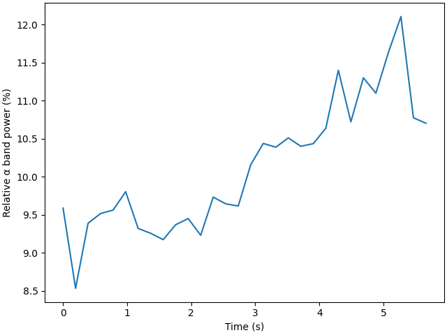
Plot in function of time🔗
We can now plot the rolling-window bandpower in function of time, using the timestamps of the last sample for each window on the X-axis. For simplicity, let’s average all channels together.
f, ax = plt.subplots(1, 1, layout="constrained")
ax.plot(times - times[0], [np.average(dp) * 100 for dp in datapoints])
ax.set_xlabel("Time (s)")
ax.set_ylabel("Relative α band power (%)")
plt.show()
Delay between 2 samples🔗
Let’s also have a look at the delay between 2 data points, i.e. the overlap between the windows.
f, ax = plt.subplots(1, 1, layout="constrained")
timedeltas = np.diff(times - times[0]) * 1000
ax.hist(timedeltas, bins=15)
ax.set_xlabel("Delay between 2 samples (ms)")
plt.show()
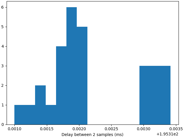
Note
Due to the low resources available on our CIs to build the documentation, some of those datapoints might have been computed with 2 acquisition window of delay instead of 1, yielding a delay between 2 samples of 2 acquisition windows instead of 1. In practice, with a large chunk size of 200 samples, we should get a delay between 2 computed time points to 200 samples, i.e. around 195.31 ms.
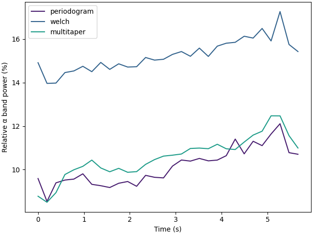
Compare power spectral density estimation methods🔗
Let’s compare both the bandpower estimation and the computation time of the different methods to estimate the power spectral density.
methods = ("periodogram", "welch", "multitaper")
with PlayerLSL(raw, chunk_size=200, name="bandpower-example", source_id=source_id):
    stream = StreamLSL(bufsize=4, name="bandpower-example", source_id=source_id)
    stream.connect(acquisition_delay=0.1, processing_flags="all")
    stream.pick("eeg").filter(1, 30)
    stream.get_data()  # reset the number of new samples after the filter is applied

    datapoints, times = {method: [] for method in methods}, []
    while stream.n_new_samples < stream.n_buffer:
        time.sleep(0.1)  # wait for the buffer to be entirely filled
    while len(datapoints[methods[0]]) != 30:
        if stream.n_new_samples == 0:
            continue  # wait for new samples
        data, ts = stream.get_data()
        for method in methods:
            bp = bandpower(data, stream.info["sfreq"], method, band=(8, 13))
            datapoints[method].append(bp)
        times.append(ts[-1])
    stream.disconnect()

f, ax = plt.subplots(1, 1, layout="constrained")
for k, method in enumerate(methods):
    ax.plot(
        times - times[0],
        [np.average(dp) * 100 for dp in datapoints[method]],
        label=method,
        color=colormaps["viridis"].colors[k * 60 + 20],
    )
ax.set_xlabel("Time (s)")
ax.set_ylabel("Relative α band power (%)")
ax.legend()
plt.show()
For the computation time and the overall loop execution speed, we need to run each method on a separate loop.
methods = ("periodogram", "welch", "multitaper")
with PlayerLSL(raw, chunk_size=200, name="bandpower-example", source_id=source_id):
    stream = StreamLSL(bufsize=4, name="bandpower-example", source_id=source_id)
    stream.connect(acquisition_delay=0.1, processing_flags="all")
    stream.pick("eeg").filter(1, 30)
    stream.get_data()  # reset the number of new samples after the filter is applied

    times = {method: [] for method in methods}
    while stream.n_new_samples < stream.n_buffer:
        time.sleep(0.1)  # wait for the buffer to be entirely filled
    for k, method in enumerate(methods):
        while len(times[methods[k]]) != 30:
            if stream.n_new_samples == 0:
                continue  # wait for new samples
            data, ts = stream.get_data()
            bp = bandpower(data, stream.info["sfreq"], method, band=(8, 13))
            times[method].append(ts[-1])
    stream.disconnect()

timedeltas = {
    method: np.diff(times[method] - times[method][0]) * 1000 for method in methods
}
timedeltas_average = {method: np.average(timedeltas[method]) for method in methods}

for method in methods:
    print(
        f"Average delay between 2 samples for {method}: "
        f"{timedeltas_average[method]:.2f} ms"
    )
Average delay between 2 samples for periodogram: 195.31 ms
Average delay between 2 samples for welch: 195.31 ms
Average delay between 2 samples for multitaper: 195.31 ms
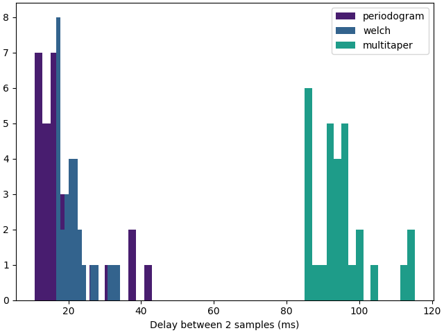
Note
For this example, the average delay between 2 estimation of the bandpower is similar between all 3 methods because we are waiting for new samples which come in chunks of 200 samples, i.e. every 195.31 ms at the sampling frequency of 1024 Hz. The figure obtained for a chunk size of 1 sample and an acquisition delay of 1 ms is shown below.
f, ax = plt.subplots(1, 1, layout="constrained")
for k, method in enumerate(methods):
    ax.hist(
        timedeltas[method],
        bins=15,
        label=method,
        color=colormaps["viridis"].colors[k * 60 + 20],
    )
ax.set_xlabel("Delay between 2 samples (ms)")
ax.legend()
plt.show()
Total running time of the script: (0 minutes 48.925 seconds)
Estimated memory usage: 258 MB