Note
Go to the end to download the full example code.
Introduction to real-time LSL streams🔗
LSL is an open-source networked middleware ecosystem to stream, receive, synchronize, and record neural, physiological, and behavioral data streams acquired from diverse sensor hardware. It reduces complexity and barriers to entry for researchers, sensor manufacturers, and users through a simple, interoperable, standardized API to connect data consumers to data producers while abstracting obstacles such as platform differences, stream discovery, synchronization and fault-tolerance. Source: LabStreamingLayer website.
In real-time applications, a server emits a data stream, and one or more clients connect
to the server to receive this data. In LSL terminology, the server is referred to as a
StreamOutlet, while the client is referred to as a
StreamInlet. The power of LSL resides in its ability to facilitate
interoperability and synchronization among streams. Clients have the capability to
connect to multiple servers, which may be running on the same or different computers
(and therefore different platforms/operating systems), and synchronize the streams
originating from these various servers.
MNE-LSL enhances the LSL API by offering a high-level interface akin to the MNE-Python API. While this tutorial concentrates on the high-level API, detailed coverage of the low-level LSL API is provided in this separate tutorial.
Concepts🔗
In essence, a real-time LSL stream can be envisioned as a perpetual recording, akin to
a mne.io.Raw instance, characterized by an indeterminate length and providing
access solely to current and preceding samples. In memory, it can be depicted as a ring
buffer, also known as a circular buffer, a data structure employing a single, unchanging
buffer size, seemingly interconnected end-to-end.
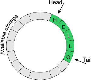
Within a ring buffer, there are two pivotal pointers:
The “head” pointer, also referred to as “start” or “read,” indicates the subsequent data block available for reading.
The “tail” pointer, known as “end” or “write,” designates the forthcoming data block to be replaced with fresh data.
In a ring buffer configuration, when the “tail” pointer aligns with the “head” pointer, data is overwritten before it can be accessed. Conversely, the “head” pointer cannot surpass the “tail” pointer; it will always lag at least one sample behind. In all cases, it falls upon the user to routinely inspect and fetch samples from the ring buffer, thereby advancing the “head” pointer.
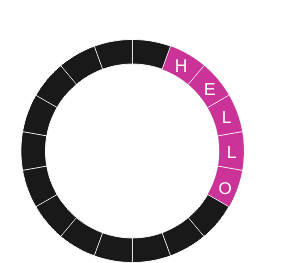
Within MNE-LSL, the StreamLSL object manages a ring buffer
internally, which is continuously refreshed with new samples. Notably, the two pointers
are concealed, with the head pointer being automatically adjusted to the latest received
sample. Given the preference for accessing the most recent information in neural,
physiological, and behavioral real-time applications, this operational approach
streamlines interaction with LSL streams and mitigates the risk of users accessing
outdated data.
Mocking an LSL stream🔗
To build real-time applications or showcase their functionalities, such as in this
tutorial, it’s essential to generate simulated LSL streams. This involves creating a
StreamOutlet and regularly sending data through it.
Within MNE-LSL, the PlayerLSL generates a simulated LSL stream
utilizing data from a mne.io.Raw file or object. This stream inherits its
description and channel specifications from the associated Info. This
information encompasses channel properties, channel locations, filters, digitization,
and SSP projectors. The PlayerLSL subsequently publishes
data at regular intervals and seamlessly loops back to the starting point once the end
of the file is reached.
import time
import uuid

from matplotlib import pyplot as plt
from mne import set_log_level

from mne_lsl.datasets import sample
from mne_lsl.player import PlayerLSL as Player
from mne_lsl.stream import StreamLSL as Stream

set_log_level("WARNING")
Note
The argument source_id can be omitted most of the time. But for reliability in
our documentation build on CIs, we assign a random unique identifier to each
mock stream created.
source_id = uuid.uuid4().hex
fname = sample.data_path() / "sample-ant-raw.fif"
player = Player(fname, chunk_size=200, source_id=source_id).start()
player.info
Once the start() is called, data is published at
regular intervals. The interval duration depends on the sampling rate and on the
number of samples pushed at once, defined by the chunk_size argument of the
PlayerLSL object.
Note
The default setting for chunk_size is 10. In real-time applications, there may
be advantages to employing smaller chunk sizes for data publication, but to build
the documentation website or to run test successfully on CIs, a larger chunk size
is used to reduce the number of push operations and improve stability.
sfreq = player.info["sfreq"]
chunk_size = player.chunk_size
interval = chunk_size / sfreq  # in seconds
print(f"Interval between 2 push operations: {interval} seconds.")
Interval between 2 push operations: 0.1953125 seconds.
A PlayerLSL can also stream annotations attached to the
mne.io.Raw object. Annotations are streamed on a second irregularly sampled
StreamOutlet. See
this separate tutorial for additional information.
Subscribing to an LSL stream🔗
With the mock LSL stream operational in the background, we can proceed to subscribe to
this stream and access both its description and the data stored within its buffer. The
StreamLSL object operates both the underlying
StreamInlet and the ring buffer, which size must be
explicitly set upon creation.
Note
A StreamLSL can connect to a single LSL stream. Thus, if
multiple LSL stream are present on the network, it’s crucial to uniquely identify
a specific LSL stream using the name, stype, and source_id arguments
of the StreamLSL object.
The stream description is automatically parsed into an mne.Info upon
connection with the method mne_lsl.stream.StreamLSL.connect().
stream = Stream(bufsize=2, source_id=source_id).connect()
stream.info
Interaction with a StreamLSL is similar to the interaction
with a mne.io.Raw. In this example, the stream is mocked from a 64 channels
EEG recording with an ANT Neuro amplifier. It includes 63 EEG, 2 EOG, 1 ECG, 1 EDA, 1
STIM channel, and uses CPz as reference.
ch_types = stream.get_channel_types(unique=True)
print(f"Channel types included: {', '.join(ch_types)}")
Channel types included: eeg, eog, gsr, ecg, stim
Operations such as channel selection, re-referencing, and filtering are performed directly on the ring buffer. For instance, we can select the EEG channels, add the missing reference channel and re-reference using a common average referencing scheme which will reduce the ring buffer to 64 channels.
Note
By design, once a re-referencing operation is performed or if at least one filter
is applied, it is not possible anymore to select a subset of channels with the
methods pick() or
drop_channels(). Note that the re-referencing is
not reversible while filters can be removed with the method
del_filter().
stream.pick("eeg")  # channel selection
assert "CPz" not in stream.ch_names  # reference absent from the data stream
stream.add_reference_channels("CPz")
stream.set_eeg_reference("average")
stream.info
Note
As for MNE-Python, methods can be chained, e.g.
stream.pick("eeg").add_reference_channels("CPz")
The ring buffer is accessed with the method get_data()
which returns both the samples and their associated timestamps. In LSL terminology, a
sample is an array of shape (n_channels,).
picks = ("Fz", "Cz", "Oz")  # channel selection
f, ax = plt.subplots(3, 1, sharex=True, constrained_layout=True)
for _ in range(3):  # acquire 3 separate window
    # figure how many new samples are available, in seconds
    winsize = stream.n_new_samples / stream.info["sfreq"]
    # retrieve and plot data
    data, ts = stream.get_data(winsize, picks=picks)
    for k, data_channel in enumerate(data):
        ax[k].plot(ts, data_channel)
    time.sleep(0.5)
for k, ch in enumerate(picks):
    ax[k].set_title(f"EEG {ch}")
ax[-1].set_xlabel("Timestamp (LSL time)")
plt.show()
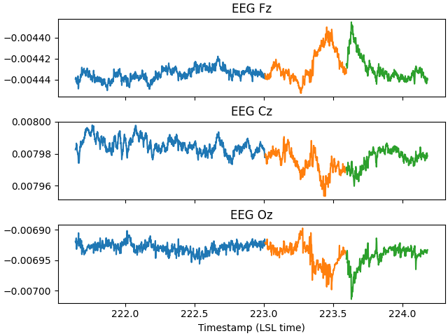
Warning
Note that the first of the 3 chunks plotted is longer. This is because
execution of the channel selection and re-referencing operations took a finite
amount of time to complete while in the background, the
StreamLSL was still acquiring new samples. Note also that
n_new_samples is reset to 0 after each call
to get_data(), but it is not reset if the “tail”
pointer overtakes the “head” pointer, in other words, it is not reset if the
number of new samples since the last get_data()
call exceeds the buffer size.
Free resources🔗
When you are done with a PlayerLSL or
StreamLSL, don’t forget to free the resources they both use
to continuously mock an LSL stream or receive new data from an LSL stream.
<Stream: OFF | MNE-LSL-Player (source: 9f9589f6e079450085c831b4e16d6cf6)>
<Player: MNE-LSL-Player | OFF | /home/runner/mne_data/MNE-LSL-data/sample/sample-ant-raw.fif>
Total running time of the script: (0 minutes 5.336 seconds)
Estimated memory usage: 296 MB