Note
Go to the end to download the full example code.
Player with annotations🔗
Annotations from a Raw object can be streamed as an event
stream by PlayerLSL. The stream is irregularly sampled and of
type 'annotations'.
A Annotations contain 3 information:
the onset of the annotation
the duration of the annotation
the description of the annotation
The PlayerLSL supports two encodings for the annotation stream,
selected with the annotations_encoding argument.
With the default annotations_encoding="one-hot", all 3 information are streamed on a
numerical stream by encoding the duration on a one-hot representation of the description
along the channels. For instance, consider a Raw object with 3
different Annotations description: 'event1', 'event2', and
'event3'. The event stream will have 3 channels, each corresponding to one of the 3
descriptions. When an annotation is streamed, its duration is encoded as the value on
its channel while the other channels remain to zero.
Note
Annotation with a duration equal to zero are special cased and yield an encoded
value of -1.
With annotations_encoding="string", only the description is streamed, on a single
'string'-typed channel named 'description'. This is convenient when a file
contains a large or variable number of unique descriptions, as the number of channels
no longer depends on the annotations present. The onset is still conveyed through the
sample timestamp, but the duration is not encoded and therefore lost. A
'string'-typed stream must be received with a StreamInlet
directly, as the StreamLSL and
EpochsStream classes only support numerical streams.
import uuid

import matplotlib.patches as mpatches
import numpy as np
from matplotlib import pyplot as plt
from mne import Annotations, create_info
from mne.io import RawArray
from mne.viz import set_browser_backend

from mne_lsl.lsl import StreamInlet, resolve_streams
from mne_lsl.player import PlayerLSL
from mne_lsl.stream import StreamLSL

annotations = Annotations(
    onset=[1, 2, 3],
    duration=[0.1, 0.2, 0.3],
    description=["event1", "event2", "event3"],
)
annotations
<Annotations | 3 segments: event1 (1), event2 (1), event3 (1)>
With the 3 annotations above, the event stream will stream the following samples:
at time
1, the annotation'event1'is pushed. The sample push isarray([[0.1, 0, 0]]), of shape (1, 3).at time
2, the annotation'event2'is pushed. The sample push isarray([[0, 0.2, 0]]), of shape (1, 3).at time
3, the annotation'event3'is pushed. The sample push isarray([[0, 0, 0.3]]), of shape (1, 3).
If more than one annotations are present in the chunk currently pushed, then a chunk
is pushed. For instance, if the annotations at time 2 and 3 are pushed at the
same time, then the chunk push is array([[0., 0.2., 0.], [0., 0., 0.3]]), of shape
(2, 3).
Example on mock signal🔗
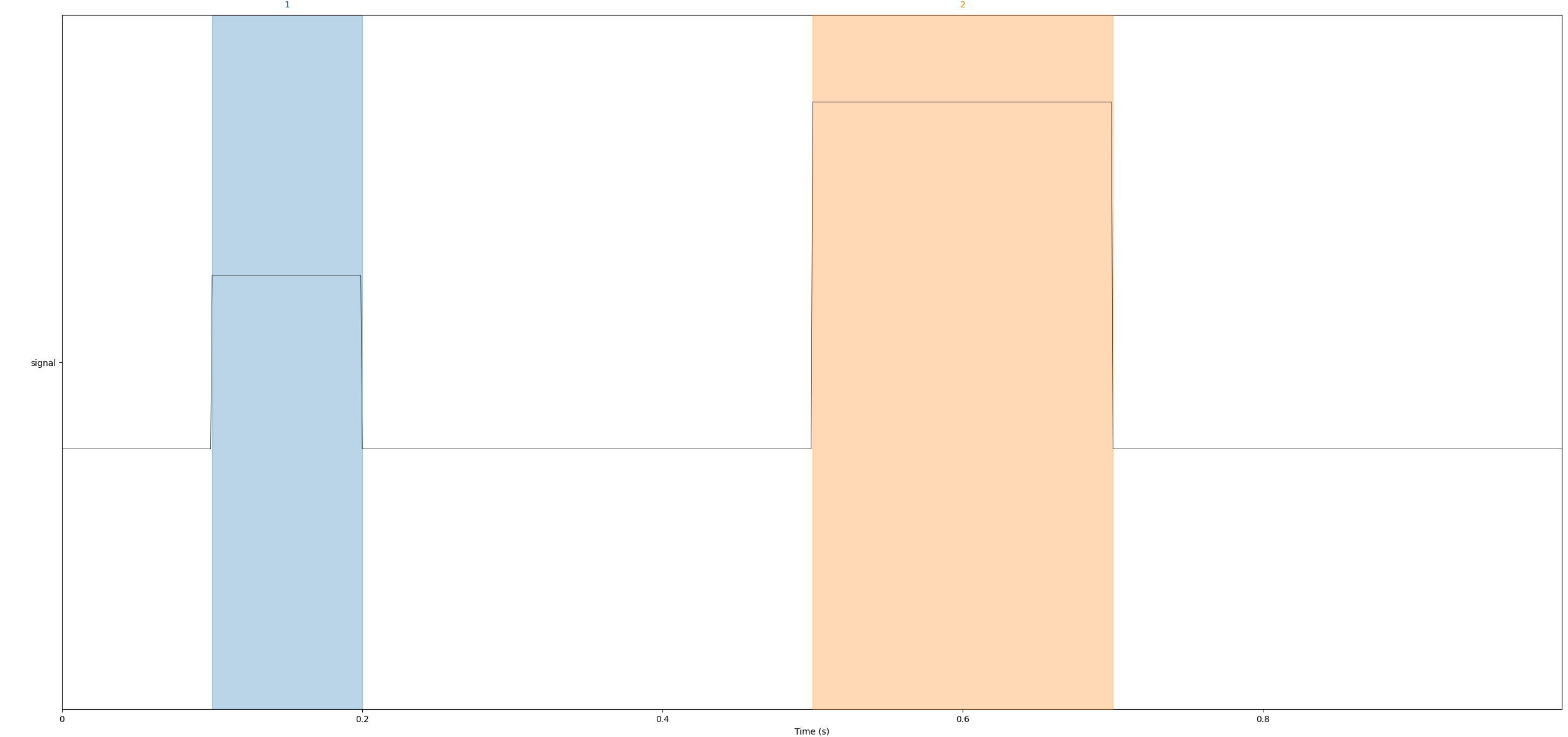
Let’s create a mock Raw object with annotations and stream both the
signal and the annotations.
data = np.zeros((1, 1000))  # 1 channel, 1000 samples
data[0, 100:200] = 1
data[0, 500:700] = 2
info = create_info(["signal"], 1000, "misc")
raw = RawArray(data, info)
annotations = Annotations(onset=[0.1, 0.5], duration=[0.1, 0.2], description=["1", "2"])
raw.set_annotations(annotations)
set_browser_backend("matplotlib")  # easier to plot with matplotlib in a documentation
raw.plot(scalings=dict(misc=2), show_scrollbars=False, show_scalebars=False)
plt.show()
Now that we have the Raw object, we can stream it with a
PlayerLSL object.
Note
Note that forcing annotations=True is not necessary since the
PlayerLSL will automatically stream annotations if they
are present in the Raw object.
Note
A chunk_size of 1 is needed here or the timestamps ts from the signal and
annotations streams are not reliable enough.
source_id = uuid.uuid4().hex
player = PlayerLSL(
    raw,
    chunk_size=1,
    name="tutorial-annots",
    source_id=source_id,
    annotations=True,
).start()
We can now acquire both streams with 2 StreamLSL objects.
stream = StreamLSL(2, name="tutorial-annots", source_id=source_id)
stream.connect(acquisition_delay=0.1, processing_flags="all")
stream.info
stream_annotations = StreamLSL(2, stype="annotations", source_id=source_id)
stream_annotations.connect(acquisition_delay=0.1, processing_flags="all")
stream_annotations.info
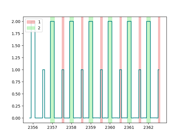
We can now acquire new samples from both streams and create a matplotlib figure to plot the signal and the annotations in real-time.
if not plt.isinteractive():
    plt.ion()
fig, ax = plt.subplots()
# add legend
colors = ["lightcoral", "lightgreen"]
patches = [
    mpatches.Patch(color=colors[k], label=ch, alpha=0.5)
    for k, ch in enumerate(stream_annotations.ch_names)
]
ax.legend(handles=patches, loc="upper left")
plt.show()

n = 0  # number of annotations
while n <= 10:
    if stream.n_new_samples == 0:
        continue

    data, ts = stream.get_data(winsize=stream.n_new_samples / stream.info["sfreq"])
    ax.plot(ts, data.squeeze(), color="teal")

    if stream_annotations.n_new_samples != 0:
        data_annotations, ts_annotations = stream_annotations.get_data(
            winsize=stream_annotations.n_new_samples
        )
        for sample, time in zip(data_annotations.T, ts_annotations, strict=True):
            k = np.where(sample != 0)[0][0]  # find the annotation
            ax.axvspan(
                time,
                time + sample[k],
                label=stream_annotations.ch_names[k],
                color=colors[k],
                alpha=0.5,
            )
        n += 1

    fig.canvas.draw()
    fig.canvas.flush_events()
Free resources🔗
When you are done with a PlayerLSL, a
StreamLSL or a EpochsStream don’t
forget to free the resources they use to continuously mock an LSL stream or
receive new data from an LSL stream.
<Stream: OFF | tutorial-annots (source: 095911768c7c4a27ae6f27365e70e2ac)>
<Stream: OFF | tutorial-annots-annotations (source: 095911768c7c4a27ae6f27365e70e2ac)>
<Player: tutorial-annots | OFF>
Streaming annotations as strings🔗
The one-hot encoding above conveys the onset, duration and description, but it creates
one channel per unique description. With many unique descriptions, e.g. a file with
hundreds of distinct markers, this yields a large and file-dependent number of
channels. If the duration is not needed, annotations_encoding="string" streams the
descriptions on a single 'string'-typed channel named 'description' instead.
A 'string'-typed stream can not be received with a
StreamLSL, which only supports numerical streams. We resolve
the annotation stream and connect to it with a StreamInlet
instead.
sinfo = [
    stream
    for stream in resolve_streams(timeout=2)
    if stream.stype == "annotations" and stream.source_id == source_id
][0]
inlet = StreamInlet(sinfo)
inlet.open_stream(timeout=5)
Each pulled sample is a list with a single element: the annotation description. The associated timestamp still encodes the onset, while the duration is lost.
descriptions = []
for _ in range(20):
    data, ts = inlet.pull_chunk(timeout=1)
    descriptions.extend(sample[0] for sample in data)
    if 4 <= len(descriptions):
        break
descriptions
['1', '2', '1', '2']
Free resources.
Similarly, when you are done with a StreamInlet, don’t forget to
free the resources they use to continuously mock an LSL stream or receive new data
from an LSL stream.
inlet.close_stream()
del inlet
player.stop()
<Player: tutorial-annots-str | OFF>
Total running time of the script: (0 minutes 14.505 seconds)
Estimated memory usage: 197 MB