mne.decoding.CSP#

class mne.decoding.CSP(n_components=4, reg=None, log=None, cov_est='concat', transform_into='average_power', norm_trace=False, cov_method_params=None, rank=None, component_order='mutual_info')[source]#

M/EEG signal decomposition using the Common Spatial Patterns (CSP).

This class can be used as a supervised decomposition to estimate spatial filters for feature extraction. CSP in the context of EEG was first described in [1]; a comprehensive tutorial on CSP can be found in [2]. Multi-class solving is implemented from [3].

Parameters:

n_componentsint (default 4)

The number of components to decompose M/EEG signals. This number should be set by cross-validation.

regfloat | str | None (default None)

If not None (same as 'empirical', default), allow regularization for covariance estimation. If float (between 0 and 1), shrinkage is used. For str values, reg will be passed as method to mne.compute_covariance().

logNone | bool (default None)

If transform_into equals 'average_power' and log is None or True, then apply a log transform to standardize features, else features are z-scored. If transform_into is 'csp_space', log must be None.

cov_est‘concat’ | ‘epoch’ (default ‘concat’)

If 'concat', covariance matrices are estimated on concatenated epochs for each class. If 'epoch', covariance matrices are estimated on each epoch separately and then averaged over each class.

transform_into‘average_power’ | ‘csp_space’ (default ‘average_power’)

If ‘average_power’ then self.transform will return the average power of each spatial filter. If 'csp_space', self.transform will return the data in CSP space.

norm_tracebool (default False)

Normalize class covariance by its trace. Trace normalization is a step of the original CSP algorithm [1] to eliminate magnitude variations in the EEG between individuals. It is not applied in more recent work [2], [3] and can have a negative impact on pattern order.

cov_method_paramsdict | None

Parameters to pass to mne.compute_covariance().

New in version 0.16.

rankNone | ‘info’ | ‘full’ | dict

This controls the rank computation that can be read from the measurement info or estimated from the data. When a noise covariance is used for whitening, this should reflect the rank of that covariance, otherwise amplification of noise components can occur in whitening (e.g., often during source localization).

None

The rank will be estimated from the data after proper scaling of different channel types.

'info'

The rank is inferred from info. If data have been processed with Maxwell filtering, the Maxwell filtering header is used. Otherwise, the channel counts themselves are used. In both cases, the number of projectors is subtracted from the (effective) number of channels in the data. For example, if Maxwell filtering reduces the rank to 68, with two projectors the returned value will be 66.

'full'

The rank is assumed to be full, i.e. equal to the number of good channels. If a Covariance is passed, this can make sense if it has been (possibly improperly) regularized without taking into account the true data rank.

dict

Calculate the rank only for a subset of channel types, and explicitly specify the rank for the remaining channel types. This can be extremely useful if you already know the rank of (part of) your data, for instance in case you have calculated it earlier.

This parameter must be a dictionary whose keys correspond to channel types in the data (e.g. 'meg', 'mag', 'grad', 'eeg'), and whose values are integers representing the respective ranks. For example, {'mag': 90, 'eeg': 45} will assume a rank of 90 and 45 for magnetometer data and EEG data, respectively.

The ranks for all channel types present in the data, but not specified in the dictionary will be estimated empirically. That is, if you passed a dataset containing magnetometer, gradiometer, and EEG data together with the dictionary from the previous example, only the gradiometer rank would be determined, while the specified magnetometer and EEG ranks would be taken for granted.

The default is None.

New in version 0.17.

component_order‘mutual_info’ | ‘alternate’ (default ‘mutual_info’)

If 'mutual_info' order components by decreasing mutual information (in the two-class case this uses a simplification which orders components by decreasing absolute deviation of the eigenvalues from 0.5 [4]). For the two-class case, 'alternate' orders components by starting with the largest eigenvalue, followed by the smallest, the second-to-largest, the second-to-smallest, and so on [2].

New in version 0.21.

See also

mne.preprocessing.Xdawn, SPoC

References

Attributes:

filters_ndarray, shape (n_channels, n_channels): If fit, the CSP components used to decompose the data, else None.
patterns_ndarray, shape (n_channels, n_channels): If fit, the CSP patterns used to restore M/EEG signals, else None.
mean_ndarray, shape (n_components,): If fit, the mean squared power for each component.
std_ndarray, shape (n_components,): If fit, the std squared power for each component.

Methods

`fit`(X, y)	Estimate the CSP decomposition on epochs.
`fit_transform`(X, y, **fit_params)	Fit to data, then transform it.
`get_params`([deep])	Get parameters for this estimator.
`plot_filters`(info[, components, average, ...])	Plot topographic filters of components.
`plot_patterns`(info[, components, average, ...])	Plot topographic patterns of components.
`set_params`(**params)	Set the parameters of this estimator.
`transform`(X)	Estimate epochs sources given the CSP filters.

fit(X, y)[source]#

Estimate the CSP decomposition on epochs.

Parameters:

Xndarray, shape (n_epochs, n_channels, n_times): The data on which to estimate the CSP.
yarray, shape (n_epochs,): The class for each epoch.

Returns:

selfinstance of CSP: Returns the modified instance.

Examples using fit:

Decoding (MVPA)

Continuous Target Decoding with SPoC

fit_transform(X, y, **fit_params)[source]#

Fit to data, then transform it.

Fits transformer to X and y with optional parameters fit_params, and returns a transformed version of X.

Parameters:

Xarray, shape (n_samples, n_features): Training set.
yarray, shape (n_samples,): Target values or class labels.
**fit_paramsdict: Additional fitting parameters passed to the fit method..

Returns:

X_newarray, shape (n_samples, n_features_new): Transformed array.

Examples using fit_transform: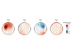

Motor imagery decoding from EEG data using the Common Spatial Pattern (CSP)

get_params(deep=True)[source]#

Get parameters for this estimator.

Parameters:

deepbool, optional: If True, will return the parameters for this estimator and contained subobjects that are estimators.

Returns:

paramsdict: Parameter names mapped to their values.

plot_filters(info, components=None, *, average=None, ch_type=None, scalings=None, sensors=True, show_names=False, mask=None, mask_params=None, contours=6, outlines='head', sphere=None, image_interp='cubic', extrapolate='auto', border='mean', res=64, size=1, cmap='RdBu_r', vlim=(None, None), cnorm=None, colorbar=True, cbar_fmt='%3.1f', units=None, axes=None, name_format='CSP%01d', nrows=1, ncols='auto', show=True)[source]#

Plot topographic filters of components.

The filters are used to extract discriminant neural sources from the measured data (a.k.a. the backward model).

Parameters:

infomne.Info

The mne.Info object with information about the sensors and methods of measurement. Used for fitting. If not available, consider using mne.create_info().

componentsfloat | array of float | None

The patterns to plot. If None, all components will be shown.

averagefloat | array_like of float, shape (n_times,) | None

The time window (in seconds) around a given time point to be used for averaging. For example, 0.2 would translate into a time window that starts 0.1 s before and ends 0.1 s after the given time point. If the time window exceeds the duration of the data, it will be clipped. Different time windows (one per time point) can be provided by passing an array-like object (e.g., [0.1, 0.2, 0.3]). If None (default), no averaging will take place.

Changed in version 1.1: Support for array-like input.

The channel type to plot. For 'grad', the gradiometers are collected in pairs and the RMS for each pair is plotted. If None the first available channel type from order shown above is used. Defaults to None.

scalingsdict | float | None

The scalings of the channel types to be applied for plotting. If None, defaults to dict(eeg=1e6, grad=1e13, mag=1e15).

sensorsbool | str

Whether to add markers for sensor locations. If str, should be a valid matplotlib format string (e.g., 'r+' for red plusses, see the Notes section of plot()). If True (the default), black circles will be used.

show_namesbool | callable()

If True, show channel names next to each sensor marker. If callable, channel names will be formatted using the callable; e.g., to delete the prefix ‘MEG ‘ from all channel names, pass the function lambda x: x.replace('MEG ', ''). If mask is not None, only non-masked sensor names will be shown.

maskndarray of bool, shape (n_channels, n_patterns) | None

Array indicating channel-pattern combinations to highlight with a distinct plotting style. Array elements set to True will be plotted with the parameters given in mask_params. Defaults to None, equivalent to an array of all False elements.

mask_paramsdict | None

Additional plotting parameters for plotting significant sensors. Default (None) equals:

dict(marker='o', markerfacecolor='w', markeredgecolor='k',
        linewidth=0, markersize=4)

contoursint | array_like

The number of contour lines to draw. If 0, no contours will be drawn. If a positive integer, that number of contour levels are chosen using the matplotlib tick locator (may sometimes be inaccurate, use array for accuracy). If array-like, the array values are used as the contour levels. The values should be in µV for EEG, fT for magnetometers and fT/m for gradiometers. If colorbar=True, the colorbar will have ticks corresponding to the contour levels. Default is 6.

outlines‘head’ | dict | None

The outlines to be drawn. If ‘head’, the default head scheme will be drawn. If dict, each key refers to a tuple of x and y positions, the values in ‘mask_pos’ will serve as image mask. Alternatively, a matplotlib patch object can be passed for advanced masking options, either directly or as a function that returns patches (required for multi-axis plots). If None, nothing will be drawn. Defaults to ‘head’.

The sphere parameters to use for the head outline. Can be array-like of shape (4,) to give the X/Y/Z origin and radius in meters, or a single float to give just the radius (origin assumed 0, 0, 0). Can also be an instance of a spherical ConductorModel to use the origin and radius from that object. If 'auto' the sphere is fit to digitization points. If 'eeglab' the head circle is defined by EEG electrodes 'Fpz', 'Oz', 'T7', and 'T8' (if 'Fpz' is not present, it will be approximated from the coordinates of 'Oz'). None (the default) is equivalent to 'auto' when enough extra digitization points are available, and (0, 0, 0, 0.095) otherwise.

New in version 0.20.

Changed in version 1.1: Added 'eeglab' option.

image_interpstr

The image interpolation to be used. Options are 'cubic' (default) to use scipy.interpolate.CloughTocher2DInterpolator, 'nearest' to use scipy.spatial.Voronoi or 'linear' to use scipy.interpolate.LinearNDInterpolator.

extrapolatestr

Options:

'box'
Extrapolate to four points placed to form a square encompassing all data points, where each side of the square is three times the range of the data in the respective dimension.
'local' (default for MEG sensors)
Extrapolate only to nearby points (approximately to points closer than median inter-electrode distance). This will also set the mask to be polygonal based on the convex hull of the sensors.
'head' (default for non-MEG sensors)
Extrapolate out to the edges of the clipping circle. This will be on the head circle when the sensors are contained within the head circle, but it can extend beyond the head when sensors are plotted outside the head circle.

Changed in version 0.21:

The default was changed to 'local' for MEG sensors.
'local' was changed to use a convex hull mask
'head' was changed to extrapolate out to the clipping circle.

New in version 1.3.

borderfloat | ‘mean’

Value to extrapolate to on the topomap borders. If 'mean' (default), then each extrapolated point has the average value of its neighbours.

New in version 0.20.

New in version 1.3.

resint

The resolution of the topomap image (number of pixels along each side).

sizefloat

Side length of each subplot in inches.

cmapmatplotlib colormap | (colormap, bool) | ‘interactive’ | None

Colormap to use. If tuple, the first value indicates the colormap to use and the second value is a boolean defining interactivity. In interactive mode the colors are adjustable by clicking and dragging the colorbar with left and right mouse button. Left mouse button moves the scale up and down and right mouse button adjusts the range. Hitting space bar resets the range. Up and down arrows can be used to change the colormap. If None, 'Reds' is used for data that is either all-positive or all-negative, and 'RdBu_r' is used otherwise. 'interactive' is equivalent to (None, True). Defaults to None.

Warning

Interactive mode works smoothly only for a small amount of topomaps. Interactive mode is disabled by default for more than 2 topomaps.

vlimtuple of length 2 | ‘joint’

Colormap limits to use. If a tuple of floats, specifies the lower and upper bounds of the colormap (in that order); providing None for either entry will set the corresponding boundary at the min/max of the data (separately for each topomap). Elements of the tuple may also be callable functions which take in a NumPy array and return a scalar. If vlim='joint', will compute the colormap limits jointly across all topomaps of the same channel type, using the min/max of the data for that channel type. Defaults to (None, None).

New in version 1.3.

cnormmatplotlib.colors.Normalize | None

How to normalize the colormap. If None, standard linear normalization is performed. If not None, vmin and vmax will be ignored. See Matplotlib docs for more details on colormap normalization, and the ERDs example for an example of its use.

New in version 1.3.

colorbarbool

Plot a colorbar in the rightmost column of the figure.

cbar_fmtstr

Formatting string for colorbar tick labels. See Format Specification Mini-Language for details.

unitsstr | None

The units to use for the colorbar label. Ignored if colorbar=False. If None the label will be “AU” indicating arbitrary units. Default is None.

axesinstance of Axes | list of Axes | None

The axes to plot to. If None, a new Figure will be created with the correct number of axes. If Axes are provided (either as a single instance or a list of axes), the number of axes provided must match the number of times provided (unless times is None).Default is None.

name_formatstr

String format for topomap values. Defaults to “CSP%01d”.

nrows, ncolsint | ‘auto’

The number of rows and columns of topographies to plot. If either nrows or ncols is 'auto', the necessary number will be inferred. Defaults to nrows=1, ncols='auto'.

New in version 1.3.

showbool

Show the figure if True.

Returns:

figinstance of matplotlib.figure.Figure: The figure.

Examples using plot_filters:

Decoding (MVPA)

plot_patterns(info, components=None, *, average=None, ch_type=None, scalings=None, sensors=True, show_names=False, mask=None, mask_params=None, contours=6, outlines='head', sphere=None, image_interp='cubic', extrapolate='auto', border='mean', res=64, size=1, cmap='RdBu_r', vlim=(None, None), cnorm=None, colorbar=True, cbar_fmt='%3.1f', units=None, axes=None, name_format='CSP%01d', nrows=1, ncols='auto', show=True)[source]#

Plot topographic patterns of components.

The patterns explain how the measured data was generated from the neural sources (a.k.a. the forward model).

Parameters:

infomne.Info

The mne.Info object with information about the sensors and methods of measurement. Used for fitting. If not available, consider using mne.create_info().

componentsfloat | array of float | None

The patterns to plot. If None, all components will be shown.

averagefloat | array_like of float, shape (n_times,) | None

Changed in version 1.1: Support for array-like input.

scalingsdict | float | None

The scalings of the channel types to be applied for plotting. If None, defaults to dict(eeg=1e6, grad=1e13, mag=1e15).

sensorsbool | str

show_namesbool | callable()

maskndarray of bool, shape (n_channels, n_patterns) | None

mask_paramsdict | None

Additional plotting parameters for plotting significant sensors. Default (None) equals:

dict(marker='o', markerfacecolor='w', markeredgecolor='k',
        linewidth=0, markersize=4)

contoursint | array_like

outlines‘head’ | dict | None

New in version 0.20.

Changed in version 1.1: Added 'eeglab' option.

image_interpstr

extrapolatestr

Options:

'box'
Extrapolate to four points placed to form a square encompassing all data points, where each side of the square is three times the range of the data in the respective dimension.
'local' (default for MEG sensors)
Extrapolate only to nearby points (approximately to points closer than median inter-electrode distance). This will also set the mask to be polygonal based on the convex hull of the sensors.
'head' (default for non-MEG sensors)
Extrapolate out to the edges of the clipping circle. This will be on the head circle when the sensors are contained within the head circle, but it can extend beyond the head when sensors are plotted outside the head circle.

Changed in version 0.21:

The default was changed to 'local' for MEG sensors.
'local' was changed to use a convex hull mask
'head' was changed to extrapolate out to the clipping circle.

New in version 1.3.

borderfloat | ‘mean’

Value to extrapolate to on the topomap borders. If 'mean' (default), then each extrapolated point has the average value of its neighbours.

New in version 0.20.

New in version 1.3.

resint

The resolution of the topomap image (number of pixels along each side).

sizefloat

Side length of each subplot in inches.

cmapmatplotlib colormap | (colormap, bool) | ‘interactive’ | None

Warning

Interactive mode works smoothly only for a small amount of topomaps. Interactive mode is disabled by default for more than 2 topomaps.

vlimtuple of length 2

New in version 1.3.

cnormmatplotlib.colors.Normalize | None

New in version 1.3.

colorbarbool

Plot a colorbar in the rightmost column of the figure.

cbar_fmtstr

Formatting string for colorbar tick labels. See Format Specification Mini-Language for details.

unitsstr | None

The units to use for the colorbar label. Ignored if colorbar=False. If None the label will be “AU” indicating arbitrary units. Default is None.

axesinstance of Axes | list of Axes | None

name_formatstr

String format for topomap values. Defaults to “CSP%01d”.

nrows, ncolsint | ‘auto’

The number of rows and columns of topographies to plot. If either nrows or ncols is 'auto', the necessary number will be inferred. Defaults to nrows=1, ncols='auto'.

New in version 1.3.

showbool

Show the figure if True.

Returns:

figinstance of matplotlib.figure.Figure: The figure.

Examples using plot_patterns:

Decoding (MVPA)

Motor imagery decoding from EEG data using the Common Spatial Pattern (CSP)

Continuous Target Decoding with SPoC

set_params(**params)[source]#

Set the parameters of this estimator.

The method works on simple estimators as well as on nested objects (such as pipelines). The latter have parameters of the form <component>__<parameter> so that it’s possible to update each component of a nested object.

Parameters:

**paramsdict: Parameters.

Returns:

instinstance: The object.

transform(X)[source]#

Estimate epochs sources given the CSP filters.

Parameters:

Xarray, shape (n_epochs, n_channels, n_times): The data.

Returns:

Xndarray: If self.transform_into == ‘average_power’ then returns the power of CSP features averaged over time and shape (n_epochs, n_sources) If self.transform_into == ‘csp_space’ then returns the data in CSP space and shape is (n_epochs, n_sources, n_times).

Examples using transform:

Motor imagery decoding from EEG data using the Common Spatial Pattern (CSP)

Examples using `mne.decoding.CSP`#

Decoding (MVPA)

Motor imagery decoding from EEG data using the Common Spatial Pattern (CSP)

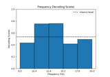
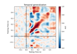
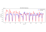
Decoding in time-frequency space using Common Spatial Patterns (CSP)

Continuous Target Decoding with SPoC

mne.decoding.CSP#

Examples using mne.decoding.CSP#

Examples using `mne.decoding.CSP`#