Note
Go to the end to download the full example code. or to run this example in your browser via Binder
Read Gowerlabs LUMO data#
LUMO is a modular, wearable, high-density diffuse optical tomography (HD-DOT) system produced by Gowerlabs. This tutorial demonstrates how to load data from LUMO, and how to utilise 3D digitisation information collected with the HD-DOT measurement.
To analyse LUMO data using MNE-NIRS, use the lumomat package to convert the native data to the SNIRF format.
HD-DOT data is often collected with individual registration of the sensor positions. In this tutorial we demonstrate how to load HD-DOT data from a LUMO device, co-register the channels to a head, and visualise the resulting channel space.
This tutorial uses the 3D graphical functionality provided by MNE-Python, to ensure you have all the required packages installed we recommend using the official MNE installers.
# sphinx_gallery_thumbnail_number = 6

# Authors: Robert Luke <code@robertluke.net>
#
# License: BSD (3-clause)

import os.path as op

import mne
from mne.datasets.testing import data_path
from mne.viz import set_3d_view
Import Gowerlabs Example File#
First, we must instruct the software where the file we wish to import resides. In this example we will use a small test file that is included in the MNE testing data set. To load your own data, replace the path stored in the fname variable by running fname = /path/to/data.snirf.
Note
The provided sample file includes only a small number of LUMO tiles, and thus channels.
import mne_nirs.io

testing_path = data_path(download=True)
fname = op.join(testing_path, "SNIRF", "GowerLabs", "lumomat-1-1-0.snirf")
We can view the path to the data by calling the variable fname.
'/home/circleci/mne_data/MNE-testing-data/SNIRF/GowerLabs/lumomat-1-1-0.snirf'
To load the file we call the function mne.io.read_raw_snirf().
raw = mne.io.read_raw_snirf(fname, preload=True)
Loading /home/circleci/mne_data/MNE-testing-data/SNIRF/GowerLabs/lumomat-1-1-0.snirf
/home/circleci/project/examples/general/plot_06_gowerlabs.py:63: RuntimeWarning: Extraction of measurement date from SNIRF file failed. The date is being set to January 1st, 2000, instead of unknownunknown
  raw = mne.io.read_raw_snirf(fname, preload=True)
Reading 0 ... 273  =      0.000 ...    27.300 secs...
And we can look at the file metadata by calling the variable raw.
raw
Visualise Data#
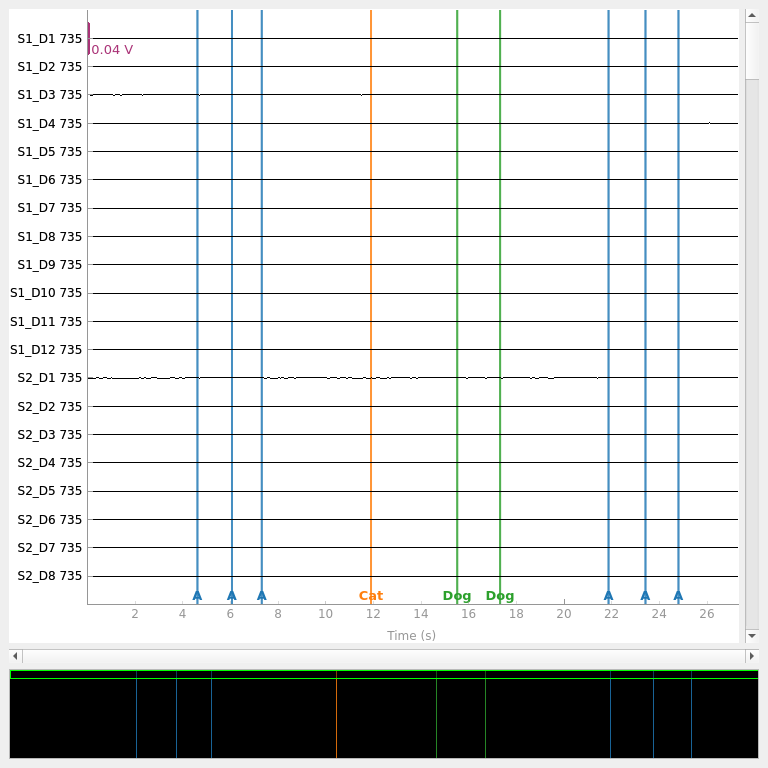
Next, we visually inspect the data to get an overview of the data quality and signal annotations.
raw.plot(duration=60)
<mne_qt_browser._pg_figure.MNEQtBrowser object at 0x7fdb498ed2d0>
We observe valid data in each channel, and note that the file includes a number of event annotations. Annotations are a flexible tool to represent events in your experiment. They can also be used to annotate other useful information such as bad segments of data, participant movements, etc. We can inspect the annotations to ensure they match what we expect from our experiment.
raw.annotations
<Annotations | 9 segments: A (6), Cat (1), Dog (2)>
The implementation of annotations varies between manufacturers. Rather than recording the onset and duration of a stimulus condition, LUMO records discrete event markers which have a nominal one second duration. Each marker can consist of an arbitrary character or string. In this sample, there were six A annotations, one Cat annotation, and two Dog annotations. We can view the specific data for each annotation by converting the annotations to a dataframe.
raw.annotations.to_data_frame()
View Optode Positions in 3D Space#
The position of optodes in 3D space is recorded and stored in the SNIRF file. These positions are stored in head coordinate frame, for a detailed overview of coordinate frames and how they are handled in MNE see Source alignment and coordinate frames.
Within the SNIRF file, the position of each optode is stored, along with scalp landmarks (“fiducials”). These positions are in an arbitrary space, and must be aligned to a scan of the participants, or a generic head.
For this data, we do not have a MRI scan of the participants head. Instead, we will align the positions to a generic head created from a collection of 40 MRI scans of real brains called fsaverage.
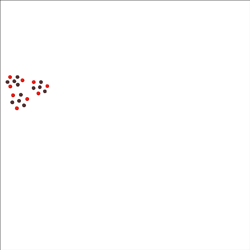
First, lets just look at the sensors in arbitrary space. Below we see that there are three LUMO tiles, each with three sources and four detectors.
subjects_dir = op.join(mne.datasets.sample.data_path(), "subjects")
mne.datasets.fetch_fsaverage(subjects_dir=subjects_dir)

brain = mne.viz.Brain(
    "fsaverage",
    subjects_dir=subjects_dir,
    alpha=0.0,
    cortex="low_contrast",
    background="w",
)
brain.add_sensors(raw.info, trans="fsaverage", fnirs=["sources", "detectors"])
brain.show_view(azimuth=130, elevation=80, distance=700)
0 files missing from root.txt in /home/circleci/mne_data/MNE-sample-data/subjects
0 files missing from bem.txt in /home/circleci/mne_data/MNE-sample-data/subjects/fsaverage
Channel types:: fnirs_cw_amplitude: 216
Coregister Optodes to Template Head#
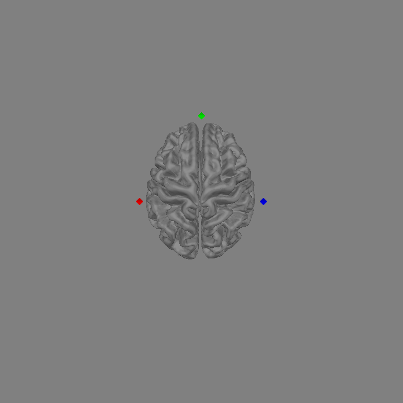
The optode locations displayed above are floating in free space and need to be aligned to our chosen head. First, lets just look at the fsaverage head that we will use.
Note
In this tutorial we use an automated code based approach
to coregistration. You can also use the MNE-Python
coregistration GUI mne.gui.coregistration().
plot_kwargs = dict(
    subjects_dir=subjects_dir,
    surfaces="brain",
    dig=True,
    eeg=[],
    fnirs=["sources", "detectors"],
    show_axes=True,
    coord_frame="head",
    mri_fiducials=True,
)

fig = mne.viz.plot_alignment(trans="fsaverage", subject="fsaverage", **plot_kwargs)
set_3d_view(figure=fig, azimuth=90, elevation=0, distance=1)
/home/circleci/project/examples/general/plot_06_gowerlabs.py:160: RuntimeWarning: Digitization points not found. Cannot plot digitization.
  fig = mne.viz.plot_alignment(trans="fsaverage", subject="fsaverage", **plot_kwargs)
This is what a head model will look like. If you have an MRI from the participant you can use freesurfer to generate the required files. For further details on generating freesurfer reconstructions see FreeSurfer MRI reconstruction.
In the figure above you can see the brain in grey. You can also see the MRI fiducial positions marked with diamonds. The nasion fiducial is marked in green, the left and right preauricular points (LPA and RPA) in red and blue respectively.
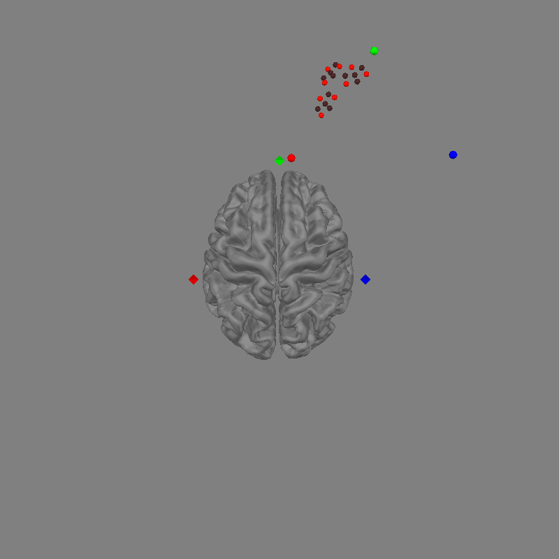
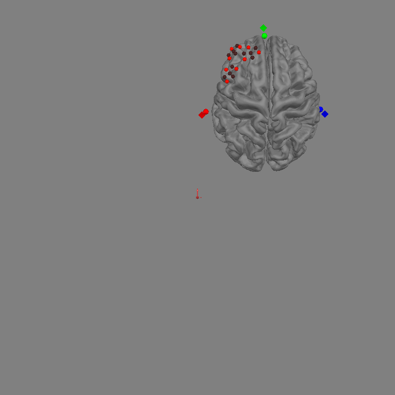
Next, we simultaneously plot the fsaverage head, and the data we wish to align to this head. This process is called coregistration and is described in several MNE-Python tutorials including Using an automated approach to coregistration.
fig = mne.viz.plot_alignment(
    raw.info, trans="fsaverage", subject="fsaverage", **plot_kwargs
)
set_3d_view(figure=fig, azimuth=90, elevation=0, distance=1)
Channel types:: fnirs_cw_amplitude: 216
In the figure above we can see the Gowerlabs optode positions and the participants digitised fiducials represented by circles. The participant digitised fiducials are a large distance from MRI fiducials on the head. To coregister the optodes to the head we will perform a rotation and translation of the optode frame to minimise the distance between the fiducials.
coreg = mne.coreg.Coregistration(
    raw.info, "fsaverage", subjects_dir, fiducials="estimated"
)
coreg.fit_fiducials(lpa_weight=1.0, nasion_weight=1.0, rpa_weight=1.0)

fig = mne.viz.plot_alignment(
    raw.info, trans=coreg.trans, subject="fsaverage", **plot_kwargs
)
set_3d_view(figure=fig, azimuth=90, elevation=0, distance=1)
Using high resolution head model in /home/circleci/mne_data/MNE-sample-data/subjects/fsaverage/bem/fsaverage-head-dense.fif
    Triangle neighbors and vertex normals...
Estimating fiducials from fsaverage.
Aligning using fiducials
Start median distance: 117.07 mm
End   median distance:   6.13 mm
Channel types:: fnirs_cw_amplitude: 216
We see in the figure above that after the fit_fiducials method was called,
the optodes are well aligned to the brain, and the distance between diamonds (MRI)
and circles (subject) fiducials is minimised. There is still some distance
between the fiducial pairs, this is because we used a generic head rather than
an individualised MRI scan. You can also mne.scale_mri() to scale
the generic MRI head.
brain = mne.viz.Brain(
    "fsaverage", subjects_dir=subjects_dir, background="w", cortex="0.5", alpha=0.3
)
brain.add_sensors(raw.info, trans=coreg.trans, fnirs=["sources", "detectors"])
brain.show_view(azimuth=90, elevation=90, distance=500)
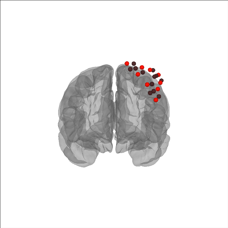
Channel types:: fnirs_cw_amplitude: 216
Apply Transformation to Raw Object#
You may wish to apply the coregistration transformation to the raw object. This can be useful if you want to save the file back to disk and not coregister again when rereading the file. Or for simpler interface using the fsaverage head.
mtg = raw.get_montage()
mtg.apply_trans(coreg.trans)
raw.set_montage(mtg)
You can then save the coregistered object.
mne_nirs.io.write_raw_snirf(raw, "raw_coregistered_to_fsaverage.snirf")
You can then load this data and use it immediately as it has already been coregistered to fsaverage.
raw_w_coreg = mne.io.read_raw_snirf("raw_coregistered_to_fsaverage.snirf")

# Now you can simply use `trans = "fsaverage"`.
brain = mne.viz.Brain(
    "fsaverage", subjects_dir=subjects_dir, background="w", cortex="0.5", alpha=0.3
)
brain.add_sensors(raw_w_coreg.info, trans="fsaverage", fnirs=["sources", "detectors"])
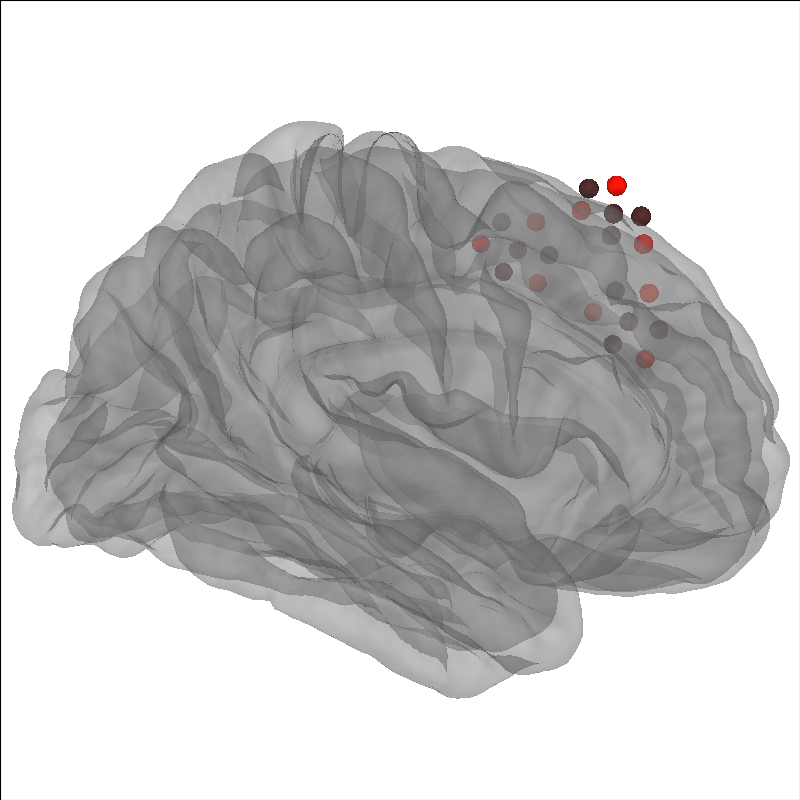
Loading /home/circleci/project/examples/general/raw_coregistered_to_fsaverage.snirf
Channel types:: fnirs_cw_amplitude: 216
Next Steps#
From here you can use your favorite analysis technique such as Waveform Averaging Analysis or GLM Analysis (Measured).
Note
HD-DOT specific tutorials are currently under development.
Total running time of the script: (0 minutes 23.423 seconds)
Estimated memory usage: 601 MB