mne.viz.Brain#
- class mne.viz.Brain(subject, hemi='both', surf='pial', title=None, cortex='classic', alpha=1.0, size=800, background='black', foreground=None, figure=None, subjects_dir=None, views='auto', *, offset='auto', interaction='trackball', units='mm', view_layout='vertical', silhouette=False, theme=None, show=True)[source]#
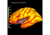
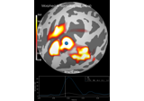
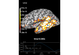
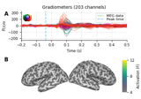
Class for visualizing a brain.
Warning
The API for this class is not currently complete. We suggest using
mne.viz.plot_source_estimates()with the PyVista backend enabled to obtain aBraininstance.- Parameters:
- subject
str Subject name in Freesurfer subjects dir.
Changed in version 1.2: This parameter was renamed from
subject_idtosubject.- hemi
str Hemisphere id (ie ‘lh’, ‘rh’, ‘both’, or ‘split’). In the case of ‘both’, both hemispheres are shown in the same window. In the case of ‘split’ hemispheres are displayed side-by-side in different viewing panes.
- surf
str FreeSurfer surface mesh name (ie ‘white’, ‘inflated’, etc.).
- title
str Title for the window.
- cortex
str,list,dict Specifies how the cortical surface is rendered. Options:
- The name of one of the preset cortex styles:
'classic'(default),'high_contrast','low_contrast', or'bone'.
- A single color-like argument to render the cortex as a single
color, e.g.
'red'or(0.1, 0.4, 1.).
- A list of two color-like used to render binarized curvature
values for gyral (first) and sulcal (second). regions, e.g.,
['red', 'blue']or[(1, 0, 0), (0, 0, 1)].
- A dict containing keys
'vmin', 'vmax', 'colormap'with values used to render the binarized curvature (where 0 is gyral, 1 is sulcal).
- A dict containing keys
Changed in version 0.24: Add support for non-string arguments.
- alpha
floatin [0, 1] Alpha level to control opacity of the cortical surface.
- size
int| array_like, shape (2,) The size of the window, in pixels. can be one number to specify a square window, or a length-2 sequence to specify (width, height).
- background
tuple(int,int,int) The color definition of the background: (red, green, blue).
- foregroundmatplotlib color
Color of the foreground (will be used for colorbars and text). None (default) will use black or white depending on the value of
background.- figure
listofFigure|None If None (default), a new window will be created with the appropriate views.
- subjects_dir
str|None If not None, this directory will be used as the subjects directory instead of the value set using the SUBJECTS_DIR environment variable.
- views
str|list View to use. Using multiple views (list) is not supported for mpl backend. See
Brain.show_viewfor valid string options.- offsetbool |
str If True, shifts the right- or left-most x coordinate of the left and right surfaces, respectively, to be at zero. This is useful for viewing inflated surface where hemispheres typically overlap. Can be “auto” (default) use True with inflated surfaces and False otherwise (Default: ‘auto’). Only used when
hemi='both'.Changed in version 0.23: Default changed to “auto”.
- interaction
str Can be “trackball” (default) or “terrain”, i.e. a turntable-style camera.
- units
str Can be ‘m’ or ‘mm’ (default).
- view_layout
str Can be “vertical” (default) or “horizontal”. When using “horizontal” mode, the PyVista backend must be used and hemi cannot be “split”.
- silhouette
dict| bool As a dict, it contains the
color,linewidth,alphaopacity anddecimate(level of decimation between 0 and 1 or None) of the brain’s silhouette to display. If True, the default values are used and if False, no silhouette will be displayed. Defaults to False.- theme
str| path-like Can be “auto”, “light”, or “dark” or a path-like to a custom stylesheet. For Dark-Mode and automatic Dark-Mode-Detection, qdarkstyle and darkdetect, respectively, are required. If None (default), the config option MNE_3D_OPTION_THEME will be used, defaulting to “auto” if it’s not found.
- showbool
Display the window as soon as it is ready. Defaults to True.
- subject
- Attributes:
Methods
add_annotation(annot[, borders, alpha, ...])Add an annotation file.
add_data(array[, fmin, fmid, fmax, thresh, ...])Display data from a numpy array on the surface or volume.
add_dipole(dipole, trans[, colors, alpha, ...])Add a quiver to render positions of dipoles.
add_foci(coords[, coords_as_verts, ...])Add spherical foci, possibly mapping to displayed surf.
add_forward(fwd, trans[, alpha, scale])Add a quiver to render positions of dipoles.
add_head([dense, color, alpha])Add a mesh to render the outer head surface.
add_label(label[, color, alpha, ...])Add an ROI label to the image.
add_sensors(info, trans[, meg, eeg, fnirs, ...])Add mesh objects to represent sensor positions.
add_skull([outer, color, alpha])Add a mesh to render the skull surface.
add_text(x, y, text[, name, color, opacity, ...])Add a text to the visualization.
add_volume_labels([aseg, labels, colors, ...])Add labels to the rendering from an anatomical segmentation.
Detect automatically fitting scaling parameters.
Clear the picking glyphs.
close()Close all figures and cleanup data structure.
Return the vertices of the picked points.
get_view([row, col, align])Get the camera orientation for a given subplot display.
help()Display the help window.
plot_time_course(hemi, vertex_id, color[, ...])Plot the vertex time course.
plot_time_line([update])Add the time line to the MPL widget.
Remove all annotations from the image.
Remove rendered data from the mesh.
Remove dipole objects from the rendered scene.
Remove forward sources from the rendered scene.
Remove head objects from the rendered scene.
Remove all the ROI labels from the image.
remove_sensors([kind])Remove sensors from the rendered scene.
Remove skull objects from the rendered scene.
remove_text([name])Remove text from the rendered scene.
Remove the volume labels from the rendered scene.
reset()Reset view, current time and time step.
Reset the camera.
Restore original scaling parameters.
save_image([filename, mode])Save view from all panels to disk.
save_movie([filename, time_dilation, tmin, ...])Save a movie (for data with a time axis).
screenshot([mode, time_viewer])Generate a screenshot of current view.
set_data_smoothing(n_steps)Set the number of smoothing steps.
set_playback_speed(speed)Set the time playback speed.
set_time(time)Set the time to display (in seconds).
set_time_interpolation(interpolation)Set the interpolation mode.
set_time_point(time_idx)Set the time point to display (can be a float to interpolate).
setup_time_viewer([time_viewer, show_traces])Configure the time viewer parameters.
show()Display the window.
show_view([view, roll, distance, row, col, ...])Orient camera to display view.
toggle_interface([value])Toggle the interface.
toggle_playback([value])Toggle time playback.
update_lut([fmin, fmid, fmax, alpha])Update the range of the color map.
Notes
The figure will publish and subscribe to the following UI events:
ColormapRange,kind="distributed_source_power"
This table shows the capabilities of each Brain backend (”✓” for full support, and “-” for partial support):
3D function:
surfer.Brain
mne.viz.Brain
✓
✓
✓
✓
✓
✓
✓
✓
✓
✓
✓
✓
✓
✓
✓
✓
✓
✓
data
✓
✓
foci
✓
labels
✓
✓
✓
✓
✓
✓
✓
✓
✓
✓
✓
✓
✓
✓
✓
✓
✓
✓
✓
✓
✓
TimeViewer
✓
✓
✓
✓
view_layout
✓
flatmaps
✓
vertex picking
✓
label picking
✓
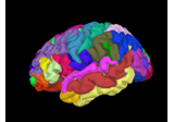
- add_annotation(annot, borders=True, alpha=1, hemi=None, remove_existing=True, color=None)[source]#
Add an annotation file.
- Parameters:
- annot
str|tuple Either path to annotation file or annotation name. Alternatively, the annotation can be specified as a
(labels, ctab)tuple per hemisphere, i.e.annot=(labels, ctab)for a single hemisphere orannot=((lh_labels, lh_ctab), (rh_labels, rh_ctab))for both hemispheres.labelsandctabshould be arrays as returned bynibabel.freesurfer.io.read_annot().- bordersbool |
int Show only label borders. If int, specify the number of steps (away from the true border) along the cortical mesh to include as part of the border definition.
- alpha
floatin [0, 1] Alpha level to control opacity. Default is 1.
- hemi
str|None If None, it is assumed to belong to the hemisphere being shown. If two hemispheres are being shown, data must exist for both hemispheres.
- remove_existingbool
If True (default), remove old annotations.
- colormatplotlib-style color
code If used, show all annotations in the same (specified) color. Probably useful only when showing annotation borders.
- annot
Examples using
add_annotation:
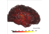
- add_data(array, fmin=None, fmid=None, fmax=None, thresh=None, center=None, transparent=False, colormap='auto', alpha=1, vertices=None, smoothing_steps=None, time=None, time_label='auto', colorbar=True, hemi=None, remove_existing=None, time_label_size=None, initial_time=None, scale_factor=None, vector_alpha=None, clim=None, src=None, volume_options=0.4, colorbar_kwargs=None, verbose=None)[source]#
Display data from a numpy array on the surface or volume.
This provides a similar interface to PySurfer, but it displays it with a single colormap. It offers more flexibility over the colormap, and provides a way to display four-dimensional data (i.e., a timecourse) or five-dimensional data (i.e., a vector-valued timecourse).
Note
fminsets the low end of the colormap, and is separate from thresh (this is a different convention from PySurfer).- Parameters:
- array
numpyarray, shape (n_vertices[, 3][, n_times]) Data array. For the data to be understood as vector-valued (3 values per vertex corresponding to X/Y/Z surface RAS), then
arraymust be have all 3 dimensions. If vectors with no time dimension are desired, consider using a singleton (e.g.,np.newaxis) to create a “time” dimension and passtime_label=None(vector values are not supported).- fmin
float Minimum value in colormap (uses real fmin if None).
- fmid
float Intermediate value in colormap (fmid between fmin and fmax if None).
- fmax
float Maximum value in colormap (uses real max if None).
- thresh
Noneorfloat Not supported yet. If not None, values below thresh will not be visible.
- center
floatorNone If not None, center of a divergent colormap, changes the meaning of fmin, fmax and fmid.
- transparentbool |
None If True: use a linear transparency between fmin and fmid and make values below fmin fully transparent (symmetrically for divergent colormaps). None will choose automatically based on colormap type.
- colormap
str,listof color, orarray Name of matplotlib colormap to use, a list of matplotlib colors, or a custom look up table (an n x 4 array coded with RBGA values between 0 and 255), the default “auto” chooses a default divergent colormap, if “center” is given (currently “icefire”), otherwise a default sequential colormap (currently “rocket”).
- alpha
floatin [0, 1] |array, shape (n_vertices,) Alpha level to control opacity of the overlay. A scalar applies globally, while a 1D array applies per-vertex opacity.
Changed in version 1.12: Added support for per-vertex alpha.
- vertices
numpyarray Vertices for which the data is defined (needed if
len(data) < nvtx).- smoothing_steps
intorNone Number of smoothing steps (smoothing is used if len(data) < nvtx) The value ‘nearest’ can be used too. None (default) will use as many as necessary to fill the surface.
- time
numpyarray Time points in the data array (if data is 2D or 3D).
- time_label
str|callable()|None Format of the time label (a format string, a function that maps floating point time values to strings, or None for no label). The default is
'auto', which will usetime=%0.2f msif there is more than one time point.- colorbarbool
Whether to add a colorbar to the figure. Can also be a tuple to give the (row, col) index of where to put the colorbar.
- hemi
str|None If None, it is assumed to belong to the hemisphere being shown. If two hemispheres are being shown, an error will be thrown.
- remove_existingbool
Not supported yet. Remove surface added by previous “add_data” call. Useful for conserving memory when displaying different data in a loop.
- time_label_size
int Font size of the time label (default 14).
- initial_time
float|None Time initially shown in the plot.
Noneto use the first time sample (default).- scale_factor
float|None(default) The scale factor to use when displaying glyphs for vector-valued data.
- vector_alpha
float|None Alpha level to control opacity of the arrows. Only used for vector-valued data. If None (default),
alphais used.- clim
dict Original clim arguments.
- srcinstance of
SourceSpaces|None The source space corresponding to the source estimate. Only necessary if the STC is a volume or mixed source estimate.
- volume_options
float|dict|None Options for volumetric source estimate plotting, with key/value pairs:
'resolution'float | NoneResolution (in mm) of volume rendering. Smaller (e.g., 1.) looks better at the cost of speed. None (default) uses the volume source space resolution, which is often something like 7 or 5 mm, without resampling.
'blending'strCan be “mip” (default) for maximum intensity projection or “composite” for composite blending using alpha values.
'alpha'float | NoneAlpha for the volumetric rendering. Defaults are 0.4 for vector source estimates and 1.0 for scalar source estimates.
'surface_alpha'float | NoneAlpha for the surface enclosing the volume(s). None (default) will use half the volume alpha. Set to zero to avoid plotting the surface.
'silhouette_alpha'float | NoneAlpha for a silhouette along the outside of the volume. None (default) will use
0.25 * surface_alpha.
'silhouette_linewidth'floatThe line width to use for the silhouette. Default is 2.
A float input (default 1.) or None will be used for the
'resolution'entry.- colorbar_kwargs
dict|None Options to pass to
pyvista.Plotter.add_scalar_bar(e.g.,dict(title_font_size=10)).- verbosebool |
str|int|None Control verbosity of the logging output. If
None, use the default verbosity level. See the logging documentation andmne.verbose()for details. Should only be passed as a keyword argument.
- array
Notes
If the data is defined for a subset of vertices (specified by the “vertices” parameter), a smoothing method is used to interpolate the data onto the high resolution surface. If the data is defined for subsampled version of the surface, smoothing_steps can be set to None, in which case only as many smoothing steps are applied until the whole surface is filled with non-zeros.
Due to a VTK alpha rendering bug,
vector_alphais clamped to be strictly < 1.Examples using
add_data:
- add_dipole(dipole, trans, colors='red', alpha=1, scales=None, *, mode='arrow')[source]#
Add a quiver to render positions of dipoles.
- Parameters:
- dipoleinstance of
Dipole Dipole object containing position, orientation and amplitude of one or more dipoles or in the forward solution.
- trans
str|dict| instance ofTransform If str, the path to the head<->MRI transform
*-trans.fiffile produced during coregistration. Can also be'fsaverage'to use the built-in fsaverage transformation.- colors
list| matplotlib-style color |None A single color or list of anything matplotlib accepts: string, RGB, hex, etc. Default red.
- alpha
floatin [0, 1] Alpha level to control opacity. Default 1.
- scales
list|float|None The size of the arrow representing the dipole in
mne.viz.Brainunits. Default 5mm.- mode“2darrow” | “arrow” | “cone” | “cylinder” | “sphere” | “oct”
The drawing mode for the dipole to render. Defaults to
"arrow".
- dipoleinstance of
Notes
New in v1.0.
Examples using
add_dipole:
- add_foci(coords, coords_as_verts=False, map_surface=None, scale_factor=1, color='white', alpha=1, name=None, hemi=None, resolution=50)[source]#
Add spherical foci, possibly mapping to displayed surf.
The foci spheres can be displayed at the coordinates given, or mapped through a surface geometry. In other words, coordinates from a volume-based analysis in MNI space can be displayed on an inflated average surface by finding the closest vertex on the white surface and mapping to that vertex on the inflated mesh.
- Parameters:
- coords
ndarray, shape (n_coords, 3) Coordinates in stereotaxic space (default) or array of vertex ids (with
coord_as_verts=True).- coords_as_vertsbool
Whether the coords parameter should be interpreted as vertex ids.
- map_surface
str|None Surface to project the coordinates to, or None to use raw coords. When set to a surface, each foci is positioned at the closest vertex in the mesh.
- scale_factor
float Controls the size of the foci spheres (relative to 1cm).
- colorcolor
A list of anything matplotlib accepts: string, RGB, hex, etc.
- alpha
floatin [0, 1] Alpha level to control opacity. Default is 1.
- name
str Internal name to use.
- hemi
str|None If None, it is assumed to belong to the hemisphere being shown. If two hemispheres are being shown, an error will be thrown.
- resolution
int The resolution of the spheres.
- coords
Examples using
add_foci: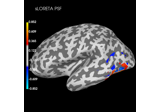
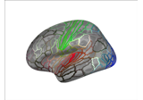
Plot point-spread functions (PSFs) and cross-talk functions (CTFs)
Plot point-spread functions (PSFs) and cross-talk functions (CTFs)
Source localization with MNE, dSPM, sLORETA, and eLORETA
Source localization with MNE, dSPM, sLORETA, and eLORETA
- add_forward(fwd, trans, alpha=1, scale=None)[source]#
Add a quiver to render positions of dipoles.
- Parameters:
- fwdinstance of
Forward The forward solution. If present, the orientations of the dipoles present in the forward solution are displayed.
- trans
str|dict| instance ofTransform If str, the path to the head<->MRI transform
*-trans.fiffile produced during coregistration. Can also be'fsaverage'to use the built-in fsaverage transformation.- alpha
floatin [0, 1] Alpha level to control opacity. Default 1.
- scale
None|float The size of the arrow representing the dipoles in
mne.viz.Brainunits. Default 1.5mm.
- fwdinstance of
Notes
New in v1.0.
- add_head(dense=True, color='gray', alpha=0.5)[source]#
Add a mesh to render the outer head surface.
- Parameters:
Notes
New in v0.24.
Examples using
add_head:
- add_label(label, color=None, alpha=1, scalar_thresh=None, borders=False, hemi=None, subdir=None)[source]#
Add an ROI label to the image.
- Parameters:
- label
str| instance ofLabel Label filepath or name. Can also be an instance of an object with attributes “hemi”, “vertices”, “name”, and optionally “color” and “values” (if scalar_thresh is not None).
- colormatplotlib-style color |
None Anything matplotlib accepts: string, RGB, hex, etc. (default “crimson”).
- alpha
floatin [0, 1] Alpha level to control opacity.
- scalar_thresh
None|float Threshold the label ids using this value in the label file’s scalar field (i.e. label only vertices with scalar >= thresh).
- bordersbool |
int Show only label borders. If int, specify the number of steps (away from the true border) along the cortical mesh to include as part of the border definition.
- hemi
str|None If None, it is assumed to belong to the hemisphere being shown.
- subdir
None|str If a label is specified as name, subdir can be used to indicate that the label file is in a sub-directory of the subject’s label directory rather than in the label directory itself (e.g. for
$SUBJECTS_DIR/$SUBJECT/label/aparc/lh.cuneus.labelbrain.add_label('cuneus', subdir='aparc')).
- label
Notes
To remove previously added labels, run Brain.remove_labels().
Examples using
add_label: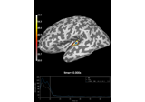
Compute Power Spectral Density of inverse solution from single epochs
Compute Power Spectral Density of inverse solution from single epochs
- add_sensors(info, trans, meg=None, eeg='original', fnirs=True, ecog=True, seeg=True, dbs=True, max_dist=0.004, *, sensor_colors=None, sensor_scales=None, verbose=None)[source]#
Add mesh objects to represent sensor positions.
- Parameters:
- info
mne.Info The
mne.Infoobject with information about the sensors and methods of measurement.- trans
str|dict| instance ofTransform If str, the path to the head<->MRI transform
*-trans.fiffile produced during coregistration. Can also be'fsaverage'to use the built-in fsaverage transformation.- meg
str|list|dict| bool |None Can be “helmet”, “sensors” or “ref” to show the MEG helmet, sensors or reference sensors respectively, or a combination like
('helmet', 'sensors')(same as None, default). True translates to('helmet', 'sensors', 'ref'). Can also be a dict to specify alpha values, e.g.{"helmet": 0.1, "sensors": 0.8}.Changed in version 1.6: Added support for specifying alpha values as a dict.
- eegbool |
str|list|dict String options are:
- “original” (default; equivalent to
True) Shows EEG sensors using their digitized locations (after transformation to the chosen
coord_frame)
- “original” (default; equivalent to
- “projected”
The EEG locations projected onto the scalp, as is done in forward modeling
Can also be a list of these options, or a dict to specify the alpha values to use, e.g.
dict(original=0.2, projected=0.8).Changed in version 1.6: Added support for specifying alpha values as a dict.
- fnirs
str|list|dict| bool |None Can be “channels”, “pairs”, “detectors”, and/or “sources” to show the fNIRS channel locations, optode locations, or line between source-detector pairs, or a combination like
('pairs', 'channels'). True translates to('pairs',). A dict can also be used to specify alpha values (but only “channels” and “pairs” will be used), e.g.dict(channels=0.2, pairs=0.7).Changed in version 1.6: Added support for specifying alpha values as a dict.
- ecogbool
If True (default), show ECoG sensors.
- seegbool
If True (default), show sEEG electrodes.
- dbsbool
If True (default), show DBS (deep brain stimulation) electrodes.
- max_dist
float The maximum distance to project a sensor to the pial surface in meters. Sensors that are greater than this distance from the pial surface will not be assigned locations. Projections can be done to the inflated or flat brain.
- sensor_colorsarray_like of color |
dict|None Colors to use for the sensor glyphs. Can be None (default) to use default colors. A dict should provide the colors (values) for each channel type (keys), e.g.:
dict(eeg=eeg_colors)
Where the value (
eeg_colorsabove) can be broadcast to an array of colors with length that matches the number of channels of that type, i.e., is compatible withmatplotlib.colors.to_rgba_array(). A few examples of this for the case above are the string"k", a list ofn_eegcolor strings, or an NumPy ndarray of shape(n_eeg, 3)or(n_eeg, 4).New in v1.6.
- sensor_scales
int|float| array_like |dict|None Scale to use for the sensor glyphs. Can be None (default) to use default scale. A dict should provide the Scale (values) for each channel type (keys), e.g.:
dict(eeg=eeg_scales)
Where the value (
eeg_scalesabove) can be broadcast to an array of values with length that matches the number of channels of that type. A few examples of this for the case above are the value10e-3, a list ofn_eegvalues, or an NumPy ndarray of shape(n_eeg,).New in v1.9.
- verbosebool |
str|int|None Control verbosity of the logging output. If
None, use the default verbosity level. See the logging documentation andmne.verbose()for details. Should only be passed as a keyword argument.
- info
Notes
New in v0.24.
Examples using
add_sensors: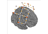
Preprocessing functional near-infrared spectroscopy (fNIRS) data
Preprocessing functional near-infrared spectroscopy (fNIRS) data
- add_skull(outer=True, color='gray', alpha=0.5)[source]#
Add a mesh to render the skull surface.
- Parameters:
Notes
New in v0.24.
- add_text(x, y, text, name=None, color=None, opacity=1.0, row=0, col=0, font_size=None, justification=None, font_file=None)[source]#
Add a text to the visualization.
- Parameters:
- x
float X coordinate.
- y
float Y coordinate.
- text
str Text to add.
- name
str Name of the text (text label can be updated using update_text()).
- color
tuple Color of the text. Default is the foreground color set during initialization (default is black or white depending on the background color).
- opacity
float Opacity of the text (default 1.0).
- row
int|None Row index of which brain to use. Default is the top row.
- col
int|None Column index of which brain to use. Default is the left-most column.
- font_size
float|None The font size to use.
- justification
str|None The text justification.
- font_file
str|None Path to an absolute path of a font file to use for rendering the text. See https://freetype.org/freetype2/docs/index.html for a list of supported font file formats.
- x
Examples using
add_text: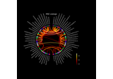
Visualize source leakage among labels using a circular graph
Visualize source leakage among labels using a circular graph
Plot point-spread functions (PSFs) and cross-talk functions (CTFs)
Plot point-spread functions (PSFs) and cross-talk functions (CTFs)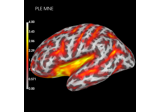
Compute spatial resolution metrics in source space
Compute spatial resolution metrics in source space
Compute spatial resolution metrics to compare MEG with EEG+MEG
Compute spatial resolution metrics to compare MEG with EEG+MEG
Source localization with MNE, dSPM, sLORETA, and eLORETA
Source localization with MNE, dSPM, sLORETA, and eLORETA
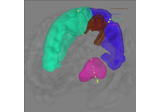
- add_volume_labels(aseg='auto', labels=None, colors=None, alpha=0.5, smooth=0.9, fill_hole_size=None, legend=None)[source]#
Add labels to the rendering from an anatomical segmentation.
- Parameters:
- aseg
str The anatomical segmentation file. Default
autousesaparc+asegif available andwmparcif not. This may be any anatomical segmentation file in the mri subdirectory of the Freesurfer subject directory.Changed in version 1.8: Added support for the new default
'auto'.- labels
list Labeled regions of interest to plot. See
mne.get_montage_volume_labels()for one way to determine regions of interest. Regions can also be chosen from the FreeSurfer LUT.- colors
list| matplotlib-style color |None A list of anything matplotlib accepts: string, RGB, hex, etc. (default FreeSurfer LUT colors).
- alpha
floatin [0, 1] Alpha level to control opacity.
- smooth
floatin [0, 1) The smoothing factor to be applied. Default 0 is no smoothing.
- fill_hole_size
int|None The size of holes to remove in the mesh in voxels. Default is None, no holes are removed. Warning, this dilates the boundaries of the surface by
fill_hole_sizenumber of voxels so use the minimal size.- legendbool |
None|dict Add a legend displaying the names of the
labels. Default (None) isTrueif the number oflabelsis 10 or fewer. Can also be a dict ofkwargsto pass topyvista.Plotter.add_legend.
- aseg
Notes
New in v0.24.
Examples using
add_volume_labels:
- property data#
Data used by time viewer and color bar widgets.
- get_view(row=0, col=0, *, align=True)[source]#
Get the camera orientation for a given subplot display.
- Parameters:
- row
int The row to use, default is the first one.
- col
int The column to check, the default is the first one.
- alignbool
If True, consider view arguments relative to canonical MRI directions (closest to MNI for the subject) rather than native MRI space. This helps when MRIs are not in standard orientation (e.g., have large rotations).
- row
- Returns:
- roll
float|None The roll of the camera rendering the view in degrees.
- distance
float| “auto” |None The distance from the camera rendering the view to the focalpoint in plot units (either m or mm). If “auto”, the bounds of visible objects will be used to set a reasonable distance.
Changed in version 1.6:
Nonewill no longer change the distance, use"auto"instead.- azimuth
float The azimuthal angle of the camera rendering the view in degrees.
- elevation
float The zenith angle of the camera rendering the view in degrees.
- focalpoint
tuple, shape (3,) |str|None The focal point of the camera rendering the view: (x, y, z) in plot units (either m or mm). When
"auto", it is set to the center of mass of the visible bounds.
- roll
- property interaction#
The interaction style.
- plot_time_line(update=True)[source]#
Add the time line to the MPL widget.
- Parameters:
- updatebool
Force an update of the plot. Defaults to True.
- save_image(filename=None, mode='rgb')[source]#
Save view from all panels to disk.
- Parameters:
Examples using
save_image: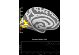
Repeated measures ANOVA on source data with spatio-temporal clustering
Repeated measures ANOVA on source data with spatio-temporal clustering
- save_movie(filename=None, time_dilation=4.0, tmin=None, tmax=None, framerate=24, interpolation=None, codec=None, bitrate=None, callback=None, time_viewer=False, **kwargs)[source]#
Save a movie (for data with a time axis).
The movie is created through the
imageiomodule. The format is determined by the extension, and additional options can be specified through keyword arguments that depend on the format, see imageio’s format page.Warning
This method assumes that time is specified in seconds when adding data. If time is specified in milliseconds this will result in movies 1000 times longer than expected.
- Parameters:
- filename
str Path at which to save the movie. The extension determines the format (e.g.,
'*.mov','*.gif', …; see theimageiodocumentation for available formats).- time_dilation
float Factor by which to stretch time (default 4). For example, an epoch from -100 to 600 ms lasts 700 ms. With
time_dilation=4this would result in a 2.8 s long movie.- tmin
float First time point to include (default: all data).
- tmax
float Last time point to include (default: all data).
- framerate
float Framerate of the movie (frames per second, default 24).
- interpolation
str|None Interpolation method (
scipy.interpolate.interp1dparameter). Must be one of'linear','nearest','zero','slinear','quadratic'or'cubic'. If None, it uses the currentbrain.interpolation, which defaults to'nearest'. Defaults to None.- codec
str|None The codec to use.
- bitrate
float|None The bitrate to use.
- callback
callable()|None A function to call on each iteration. Useful for status message updates. It will be passed keyword arguments
frameandn_frames.- time_viewerbool
If True, include time viewer traces. Only used if
time_viewer=Trueandseparate_canvas=False.- **kwargs
dict Specify additional options for
imageio.
- filename
- screenshot(mode='rgb', time_viewer=False)[source]#
Generate a screenshot of current view.
- Parameters:
- Returns:
- screenshot
array Image pixel values.
- screenshot
Examples using
screenshot:
- set_data_smoothing(n_steps)[source]#
Set the number of smoothing steps.
- Parameters:
- n_steps
int Number of smoothing steps.
- n_steps
- set_playback_speed(speed)[source]#
Set the time playback speed.
- Parameters:
- speed
float The speed of the playback.
- speed
- set_time(time)[source]#
Set the time to display (in seconds).
- Parameters:
- time
float The time to show, in seconds.
- time
Examples using
set_time:
- set_time_interpolation(interpolation)[source]#
Set the interpolation mode.
- Parameters:
- interpolation
str|None Interpolation method (
scipy.interpolate.interp1dparameter). Must be one of'linear','nearest','zero','slinear','quadratic'or'cubic'.
- interpolation
- setup_time_viewer(time_viewer=True, show_traces=True)[source]#
Configure the time viewer parameters.
- Parameters:
Notes
The keyboard shortcuts are the following:
‘?’: Display help window ‘i’: Toggle interface ‘s’: Apply auto-scaling ‘r’: Restore original clim ‘c’: Clear all traces ‘n’: Shift the time forward by the playback speed ‘b’: Shift the time backward by the playback speed ‘Space’: Start/Pause playback ‘Up’: Decrease camera elevation angle ‘Down’: Increase camera elevation angle ‘Left’: Decrease camera azimuth angle ‘Right’: Increase camera azimuth angle
- show_view(view=None, roll=None, distance=None, *, row=None, col=None, hemi=None, align=True, azimuth=None, elevation=None, focalpoint=None, update=True, verbose=None)[source]#
Orient camera to display view.
- Parameters:
- view
str|None The name of the view to show (e.g. “lateral”). Other arguments take precedence and modify the camera starting from the
view. SeeBrain.show_viewfor valid string shortcut options.- roll
float|None The roll of the camera rendering the view in degrees.
- distance
float| “auto” |None The distance from the camera rendering the view to the focalpoint in plot units (either m or mm). If “auto”, the bounds of visible objects will be used to set a reasonable distance.
Changed in version 1.6:
Nonewill no longer change the distance, use"auto"instead.- row
int|None The row to set. Default all rows.
- col
int|None The column to set. Default all columns.
- hemi
str|None Which hemi to use for view lookup (when in “both” mode).
- alignbool
If True, consider view arguments relative to canonical MRI directions (closest to MNI for the subject) rather than native MRI space. This helps when MRIs are not in standard orientation (e.g., have large rotations).
- azimuth
float The azimuthal angle of the camera rendering the view in degrees.
- elevation
float The zenith angle of the camera rendering the view in degrees.
- focalpoint
tuple, shape (3,) |str|None The focal point of the camera rendering the view: (x, y, z) in plot units (either m or mm). When
"auto", it is set to the center of mass of the visible bounds.- updatebool
Force an update of the plot. Defaults to True.
New in v1.6.
- verbosebool |
str|int|None Control verbosity of the logging output. If
None, use the default verbosity level. See the logging documentation andmne.verbose()for details. Should only be passed as a keyword argument.
- view
Notes
The builtin string views are the following perspectives, based on the RAS convention. If not otherwise noted, the view will have the top of the brain (superior, +Z) in 3D space shown upward in the 2D perspective:
'lateral'From the left or right side such that the lateral (outside) surface of the given hemisphere is visible.
'medial'From the left or right side such that the medial (inside) surface of the given hemisphere is visible (at least when in split or single-hemi mode).
'rostral'From the front.
'caudal'From the rear.
'dorsal'From above, with the front of the brain pointing up.
'ventral'From below, with the front of the brain pointing up.
'frontal'From the front and slightly lateral, with the brain slightly tilted forward (yielding a view from slightly above).
'parietal'From the rear and slightly lateral, with the brain slightly tilted backward (yielding a view from slightly above).
'axial'From above with the brain pointing up (same as
'dorsal').'sagittal'From the right side.
'coronal'From the rear.
Three letter abbreviations (e.g.,
'lat') of all of the above are also supported.Examples using
show_view:
Plot point-spread functions (PSFs) and cross-talk functions (CTFs)
Plot point-spread functions (PSFs) and cross-talk functions (CTFs)
Preprocessing functional near-infrared spectroscopy (fNIRS) data
Preprocessing functional near-infrared spectroscopy (fNIRS) data
Repeated measures ANOVA on source data with spatio-temporal clustering
Repeated measures ANOVA on source data with spatio-temporal clustering
- property time_interpolation#
The interpolation mode.
Examples using mne.viz.Brain#
Compute source level time-frequency timecourses using a DICS beamformer
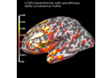
Compute evoked ERS source power using DICS, LCMV beamformer, and dSPM
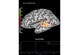
Compute MNE inverse solution on evoked data with a mixed source space
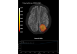
Compute source power estimate by projecting the covariance with MNE
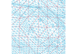
Visualize source leakage among labels using a circular graph
Plot point-spread functions (PSFs) and cross-talk functions (CTFs)
Compute spatial resolution metrics in source space
Compute spatial resolution metrics to compare MEG with EEG+MEG
Compute Power Spectral Density of inverse solution from single epochs
Compute source power spectral density (PSD) of VectorView and OPM data
Source localization with MNE, dSPM, sLORETA, and eLORETA
The role of dipole orientations in distributed source localization
EEG source localization given electrode locations on an MRI
Working with CTF data: the Brainstorm auditory dataset
Preprocessing functional near-infrared spectroscopy (fNIRS) data
Preprocessing optically pumped magnetometer (OPM) MEG data
Permutation t-test on source data with spatio-temporal clustering
2 samples permutation test on source data with spatio-temporal clustering
Repeated measures ANOVA on source data with spatio-temporal clustering