Mayer Wave Parametrisation

Cite the FOOOF authors

This tutorial is only possible due to the excellent and generous work of the FOOOF authors. Please visit their site https://fooof-tools.github.io/fooof. Also be sure to cite their various papers:

Donoghue, Thomas, et al. “Parameterizing neural power spectra into periodic and aperiodic components.” Nature neuroscience 23.12 (2020): 1655-1665.

Donoghue, Thomas, Julio Dominguez, and Bradley Voytek. “Electrophysiological frequency band ratio measures conflate periodic and aperiodic neural activity.” Eneuro 7.6 (2020).

Mayer waves are spontaneous oscillations in arterial blood pressure with a frequency of ~0.1 Hz (Ghali and Ghali, 2020; Julien, 2006; Yucel, 2016). Mayer waves are not easily removed from hemodynamic signatures of brain activity as they tend to occur on a time course often confounded with the frequency of a sensory task, for example, and/or the cortical hemodynamic response to that task.

This example demonstrates how to use the Fitting Oscillations & One Over F (FOOOF) [1] method to quanitfy Mayer wave parameters in fNIRS data. This is based on the description provided in [2].

This tutorial is heavily based on the tutorials provided by the FOOOF authors over at https://fooof-tools.github.io/fooof. You should read their excellent documentation. Their work should be considered the primary resource, and this is just an example of how to apply it to fNIRS data for the purpose of extracting Mayer waves oscillation parameters.

# Authors: Robert Luke <mail@robertluke.net>
#
# License: BSD (3-clause)

import os
import mne
import numpy as np
import matplotlib.pyplot as plt

from mne.preprocessing.nirs import optical_density, beer_lambert_law

from mne_nirs.channels import get_long_channels
from mne_nirs.preprocessing import quantify_mayer_fooof

from fooof import FOOOF

/home/circleci/project/examples/general/plot_40_mayer.py:58: DeprecationWarning:
The `fooof` package is being deprecated and replaced by the `specparam` (spectral parameterization) package.
This version of `fooof` (1.1) is fully functional, but will not be further updated.
New projects are recommended to update to using `specparam` (see Changelog for details).
  from fooof import FOOOF

Import and preprocess data

We read in the data and convert to haemoglobin concentration.

fnirs_data_folder = mne.datasets.fnirs_motor.data_path()
fnirs_raw_dir = os.path.join(fnirs_data_folder, 'Participant-1')
raw = mne.io.read_raw_nirx(fnirs_raw_dir, verbose=True).load_data()

raw = optical_density(raw)
raw.resample(2)
raw = beer_lambert_law(raw, ppf=0.1)
raw = raw.pick(picks="hbo")
raw = get_long_channels(raw, min_dist=0.025, max_dist=0.045)
raw

Loading /home/circleci/mne_data/MNE-fNIRS-motor-data/Participant-1

General

Measurement date	November 02, 2019 13:16:16 GMT
Experimenter	Unknown
Participant	P1

Channels

Digitized points	31 points
Good channels	20 Oxyhemoglobin
Bad channels	None
EOG channels	Not available
ECG channels	Not available

Data

Sampling frequency	2.00 Hz
Highpass	0.00 Hz
Lowpass	1.00 Hz
Filenames	Participant-1
Duration	00:49:34 (HH:MM:SS)

Process data with FOOOF

Next we estimate the power spectral density of the data and pass this to the FOOOF algorithm.

I recommend using the FOOOF algorithm as provided by the authors rather than reimplementation or custom plotting etc. Their code is of excellent quality, well maintained, thoroughly documented, and they have considered many edge cases.

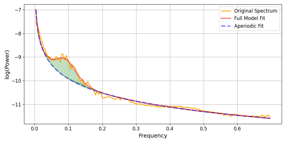
Below we plot the spectrum of the data, the FOOOF fit of oscillations, and aperiodic component. Note the bump at 0.1 Hz that reflects the Mayer wave activity.

Note that the activity is not a perfect peak at 0.1 Hz, but is spread across neighbouring frequencies. Additionally, the peak does not occur at exactly 0.1 Hz, but instead seems to peak at approximately 0.09 Hz. The shaded area illustrates the oscillation fitted by the FOOOF algorithm, it matches well to the data.

def scale_up_spectra(spectra, freqs):
    """
    FOOOF requires the frequency values to be higher than the fNIRS data
    permits, so we scale the values up by 10 here, and then will scale
    the frequency values down by 10 later.
    """
    freqs = freqs * 10
    return spectra, freqs

# Prepare data for FOOOF
psd = raw.compute_psd(
    fmin=0.001, fmax=1.0, tmin=0, tmax=None, n_overlap=300, n_fft=600)
spectra, freqs = psd.get_data(return_freqs=True)
spectra, freqs = scale_up_spectra(spectra, freqs)

# Specify the model, note that frequency values here are times 10
fm = FOOOF(peak_width_limits=(0.5, 12.0))
# Set the frequency range to fit the model, again these are times 10
freq_range = [0.001, 7]

fm.fit(freqs, np.mean(spectra, axis=0), freq_range)

fig, axs = plt.subplots(1, 1, figsize=(10, 5))
fm.plot(plot_peaks='shade', data_kwargs={'color': 'orange'}, ax=axs)
# Correct for x10 scaling above
plt.xticks([0, 1, 2, 3, 4, 5, 6], [0.0, 0.1, 0.2, 0.3, 0.4, 0.5, 0.6])

([<matplotlib.axis.XTick object at 0x7fb734976770>, <matplotlib.axis.XTick object at 0x7fb734976a10>, <matplotlib.axis.XTick object at 0x7fb629aaddb0>, <matplotlib.axis.XTick object at 0x7fb7372e57b0>, <matplotlib.axis.XTick object at 0x7fb78ffe6680>, <matplotlib.axis.XTick object at 0x7fb7372e5d20>, <matplotlib.axis.XTick object at 0x7fb78ffe69e0>], [Text(0, 0, '0.0'), Text(1, 0, '0.1'), Text(2, 0, '0.2'), Text(3, 0, '0.3'), Text(4, 0, '0.4'), Text(5, 0, '0.5'), Text(6, 0, '0.6')])

Use MNE-NIRS to quantify Mayer wave oscillation

MNE-NIRS provides a convenient function to estimate the Mayer wave parameters that takes care of the frequency scaling and selects the component most likely associated with the Mayer wave. It returns this data in a pandas dataframe for your convenience. It uses the FOOOF algorithm under the hood, so ensure you cite the original authors if you use this function.

quantify_mayer_fooof(raw.pick("hbo"), extra_df_fields={"Study": "Online tutorial"})

	Centre Frequency	Bandwidth	Power	Chromaphore	Study
0	0.090168	0.069643	0.763865	hbo	Online tutorial

Conclusion

We have demonstrated how to use the FOOOF algorithm for quantifying Mayer wave parameters, and highlighted the quantify_mayer_fooof for conveniently applying this analysis to fNIRS data with MNE-NIRS.

An example measurement illustrated what the presence of a Mayer wave looks like with a power spectral density. The measurement also illustrated that the Mayer wave is not a perfect sinusoid, as evidenced by the broad spectral content. Further, the example illustrated that the Mayer wave is not always precisely locked to 0.1 Hz, both visual inspection and FOOOF quantification indicate a 0.09 Hz centre frequency.

See the article Luke (2021) [2] for further details on this analysis approach, and normative data from over 300 fNIRS measurements. This article also demonstrates that using short-channel systemic component correction algorithms can reduce the Mayer wave component in the signal (see also Yucel 2016). See both the GLM tutorial and signal enhancement tutorial for how to use short channels in either a GLM or averaging analysis with MNE-NIRS.

Bibliography

[1]

Thomas Donoghue, Matar Haller, Erik J Peterson, Paroma Varma, Priyadarshini Sebastian, Richard Gao, Torben Noto, Antonio H Lara, Joni D Wallis, Robert T Knight, and others. Parameterizing neural power spectra into periodic and aperiodic components. Nature neuroscience, 23(12):1655–1665, 2020.

[2] (1,2)

Robert Luke, Maureen Shader, and David McAlpine. Characterization of mayer-wave oscillations in functional near-infrared spectroscopy using a physiologically informed model of the neural power spectra. Neurophotonics, 8(4):041001–041001, 2021. doi:10.1117/1.NPh.8.4.041001.

Estimated memory usage: 9 MB