Note
Go to the end to download the full example code. or to run this example in your browser via Binder
GLM FIR Analysis#
In this example we analyse data from a real multi-channel functional near-infrared spectroscopy (fNIRS) experiment (see GLM Analysis (Simulated) for a simplified simulated analysis). The experiment consists of three conditions: 1) tapping with the left hand, 2) tapping with the right hand, and 3) a control condition where the participant does nothing.
In this tutorial the morphology of an fNIRS response is obtained using a Finite Impulse Response (FIR) GLM analysis. An alternative epoching-style analysis on the same data can be viewed in the waveform analysis example. See Luke et al (2021) for a comparison of the epoching and GLM FIR approaches.
This tutorial only examines the tapping with the right hand condition to simplify explanation and minimise computation time. The reader is invited to expand the code to also analyse the other conditions.
This GLM analysis is a wrapper over the excellent Nilearn GLM.
Note
This is an advanced tutorial and requires knowledge of pandas and numpy. I plan to write some functions to make this more convenient in the future.
Note
The sample rate used in this example is set to 0.5 Hz. This is to ensure that the code can run on the continuous integration servers. You may wish to increase the sample rate by adjusting resample below for your own analysis.
Note
This tutorial uses data stored using the BIDS format [1].
MNE-Python allows you to process fNIRS data that is not in BIDS format.
Simply modify the read_raw_ function to match your data type.
See data importing tutorial to learn how
to use your data with MNE-Python.
# sphinx_gallery_thumbnail_number = 1

# Authors: Robert Luke <mail@robertluke.net>
#
# License: BSD (3-clause)

# Import common libraries
# Import Plotting Library
import matplotlib.pyplot as plt
import numpy as np
import pandas as pd

# Import StatsModels
import statsmodels.formula.api as smf

# Import MNE processing
from mne.preprocessing.nirs import beer_lambert_law, optical_density

# Import MNE-BIDS processing
from mne_bids import BIDSPath, read_raw_bids

from mne_nirs.channels import get_long_channels, get_short_channels
from mne_nirs.datasets import fnirs_motor_group
from mne_nirs.experimental_design import make_first_level_design_matrix

# Import MNE-NIRS processing
from mne_nirs.statistics import run_glm, statsmodels_to_results
Define FIR analysis#
This code runs a FIR GLM analysis. It fits a FIR for each sample from the onset of a trigger. We specify here that 10 FIR delays should be used. This results in values being estimated for 10 delay steps. Due to the chosen sample rate of 0.5 Hz, these delays correspond to 0, 2, 4… seconds from the onset of the stimulus.
def analysis(fname, ID):
    raw_intensity = read_raw_bids(bids_path=fname, verbose=False)
    # Delete annotation labeled 15, as these just signify the experiment start and end.
    raw_intensity.annotations.delete(raw_intensity.annotations.description == "15.0")
    # sanitize event names
    raw_intensity.annotations.description[:] = [
        d.replace("/", "_") for d in raw_intensity.annotations.description
    ]

    # Convert signal to haemoglobin and just keep hbo
    raw_od = optical_density(raw_intensity)
    raw_haemo = beer_lambert_law(raw_od, ppf=0.1)
    raw_haemo.resample(0.5, npad="auto")

    # Cut out just the short channels for creating a GLM regressor
    short_chans = get_short_channels(raw_haemo)
    raw_haemo = get_long_channels(raw_haemo)

    # Create a design matrix
    design_matrix = make_first_level_design_matrix(
        raw_haemo,
        hrf_model="fir",
        stim_dur=1.0,
        fir_delays=range(10),
        drift_model="cosine",
        high_pass=0.01,
        oversampling=1,
    )
    # Add short channels as regressor in GLM
    for chan in range(len(short_chans.ch_names)):
        design_matrix[f"short_{chan}"] = short_chans.get_data(chan).T

    # Run GLM
    glm_est = run_glm(raw_haemo, design_matrix)

    # Create a single ROI that includes all channels for example
    rois = dict(AllChannels=range(len(raw_haemo.ch_names)))
    # Calculate ROI for all conditions
    conditions = design_matrix.columns
    # Compute output metrics by ROI
    df_ind = glm_est.to_dataframe_region_of_interest(rois, conditions)

    df_ind["ID"] = ID
    df_ind["theta"] = [t * 1.0e6 for t in df_ind["theta"]]

    return df_ind, raw_haemo, design_matrix
Run analysis#
The analysis is run on each individual subject measurement. The individual results are then appended to a dataframe for group-level analysis below.
df = pd.DataFrame()

for sub in range(1, 6):  # Loop from first to fifth subject
    ID = "%02d" % sub  # Tidy the subject name

    # Create path to file based on experiment info
    bids_path = BIDSPath(
        subject=ID,
        task="tapping",
        root=fnirs_motor_group.data_path(),
        datatype="nirs",
        suffix="nirs",
        extension=".snirf",
    )

    df_individual, raw, dm = analysis(bids_path, ID)

    df = pd.concat([df, df_individual])
Reading 0 ... 23238  =      0.000 ...  2974.464 secs...
Reading 0 ... 18877  =      0.000 ...  2416.256 secs...
Reading 0 ... 18874  =      0.000 ...  2415.872 secs...
Reading 0 ... 23120  =      0.000 ...  2959.360 secs...
Reading 0 ... 23006  =      0.000 ...  2944.768 secs...
Tidy the dataframe#
For simplicity we only examine the data from the right hand tapping condition. The code below retains only the relevant information from the dataframe and design matrix for the following statistical analysis.
# Keep only tapping and FIR delay information in the dataframe
# I.e., for this example we are not interest in the drift coefficients,
# short channel information, or control conditions.
df["isTapping"] = ["Tapping_Right" in n for n in df["Condition"]]
df["isDelay"] = ["delay" in n for n in df["Condition"]]
df = df.query("isDelay in [True]")
df = df.query("isTapping in [True]")
# Make a new column that stores the condition name for tidier model below
df.loc[:, "TidyCond"] = ""
df.loc[df["isTapping"] == True, "TidyCond"] = "Tapping"  # noqa: E712
# Finally, extract the FIR delay in to its own column in data frame
df.loc[:, "delay"] = [n.split("_")[-1] for n in df.Condition]

# To simplify this example we will only look at the right hand tapping
# condition so we now remove the left tapping conditions from the
# design matrix and GLM results
dm_cols_not_left = np.where(["Right" in c for c in dm.columns])[0]
dm = dm[[dm.columns[i] for i in dm_cols_not_left]]
Run group-level model#
A linear mixed effects (LME) model is used to determine the effect of FIR delay for each chromophore on the evoked response with participant (ID) as a random variable.
lme = smf.mixedlm("theta ~ -1 + delay:TidyCond:Chroma", df, groups=df["ID"]).fit()

# The model is summarised below, and is not displayed here.
# You can display the model output using: lme.summary()
Summarise group-level findings#
Next the values from the model above are extracted into a dataframe for more convenient analysis below. A subset of the results is displayed, illustrating the estimated coefficients for oxyhaemoglobin (HbO) for the right hand tapping condition.
# Create a dataframe from LME model for plotting below
df_sum = statsmodels_to_results(lme)
df_sum["delay"] = [int(n) for n in df_sum["delay"]]
df_sum = df_sum.sort_values("delay")

# Print the result for the oxyhaemoglobin data in the tapping condition
df_sum.query("TidyCond in ['Tapping']").query("Chroma in ['hbo']")
Note in the output above that there are 10 FIR delays. A coefficient estimate has been calculated for each delay. These coefficients must be multiplied by the FIR function to obtain the morphology of the fNIRS response.
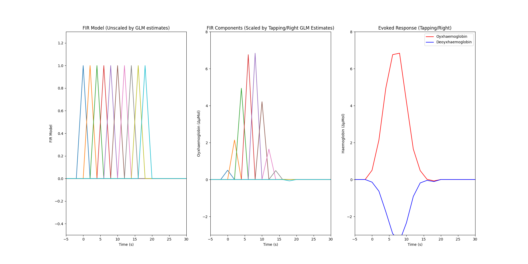
Plot the response from a single condition#
Finally we create a plot with three facets. The first facet illustrates the FIR model that was used in the GLM analysis, the model results displayed in the table above indicate the scaling values that should be applied to this model so that it best describes the measured data. The second facet illustrates the estimated amplitude of each FIR component for the right hand tapping condition for the oxyhaemoglobin data, it is obtained by multiplying the FIR model by the estimated coefficients from the GLM output. The third facet illustrates the overall estimated response for each chromophore and is calculated by summing all the individual FIR components per chromophore (HbR not shown in first two facets).
fig, axes = plt.subplots(nrows=1, ncols=3, figsize=(20, 10))

# Extract design matrix columns that correspond to the condition of interest
dm_cond_idxs = np.where(["Tapping" in n for n in dm.columns])[0]
dm_cond = dm[[dm.columns[i] for i in dm_cond_idxs]]

# Extract the corresponding estimates from the lme dataframe for hbo
df_hbo = df_sum.query("TidyCond in ['Tapping']").query("Chroma in ['hbo']")
vals_hbo = [float(v) for v in df_hbo["Coef."]]
dm_cond_scaled_hbo = dm_cond * vals_hbo

# Extract the corresponding estimates from the lme dataframe for hbr
df_hbr = df_sum.query("TidyCond in ['Tapping']").query("Chroma in ['hbr']")
vals_hbr = [float(v) for v in df_hbr["Coef."]]
dm_cond_scaled_hbr = dm_cond * vals_hbr

# Extract the time scale for plotting.
# Set time zero to be the onset of the finger tapping.
index_values = dm_cond_scaled_hbo.index - np.ceil(raw.annotations.onset[0])
index_values = np.asarray(index_values)

# Plot the result
axes[0].plot(index_values, np.asarray(dm_cond))
axes[1].plot(index_values, np.asarray(dm_cond_scaled_hbo))
axes[2].plot(index_values, np.sum(dm_cond_scaled_hbo, axis=1), "r")
axes[2].plot(index_values, np.sum(dm_cond_scaled_hbr, axis=1), "b")

# Format the plot
for ax in range(3):
    axes[ax].set_xlim(-5, 30)
    axes[ax].set_xlabel("Time (s)")
axes[0].set_ylim(-0.5, 1.3)
axes[1].set_ylim(-3, 8)
axes[2].set_ylim(-3, 8)
axes[0].set_title("FIR Model (Unscaled by GLM estimates)")
axes[1].set_title("FIR Components (Scaled by Tapping/Right GLM Estimates)")
axes[2].set_title("Evoked Response (Tapping/Right)")
axes[0].set_ylabel("FIR Model")
axes[1].set_ylabel("Oyxhaemoglobin (ΔμMol)")
axes[2].set_ylabel("Haemoglobin (ΔμMol)")
axes[2].legend(["Oyxhaemoglobin", "Deoyxhaemoglobin"])
<matplotlib.legend.Legend object at 0x7fdba03157b0>
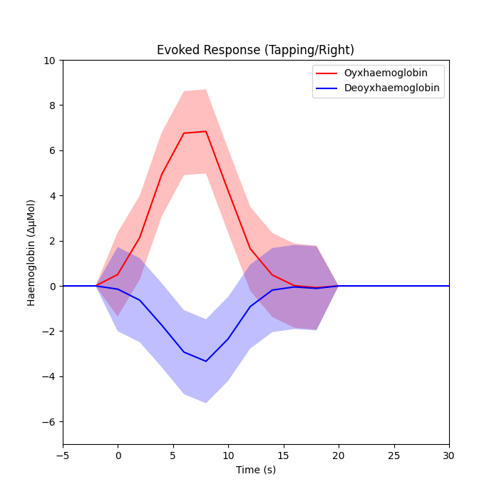
Plot the response with confidence intervals#
# We can also extract the 95% confidence intervals of the estimates too
l95_hbo = [float(v) for v in df_hbo["[0.025"]]  # lower estimate
u95_hbo = [float(v) for v in df_hbo["0.975]"]]  # upper estimate
dm_cond_scaled_hbo_l95 = dm_cond * l95_hbo
dm_cond_scaled_hbo_u95 = dm_cond * u95_hbo
l95_hbr = [float(v) for v in df_hbr["[0.025"]]  # lower estimate
u95_hbr = [float(v) for v in df_hbr["0.975]"]]  # upper estimate
dm_cond_scaled_hbr_l95 = dm_cond * l95_hbr
dm_cond_scaled_hbr_u95 = dm_cond * u95_hbr

fig, axes = plt.subplots(nrows=1, ncols=1, figsize=(7, 7))

# Plot the result
axes.plot(index_values, np.sum(dm_cond_scaled_hbo, axis=1), "r")
axes.plot(index_values, np.sum(dm_cond_scaled_hbr, axis=1), "b")
axes.fill_between(
    index_values,
    np.asarray(np.sum(dm_cond_scaled_hbo_l95, axis=1)),
    np.asarray(np.sum(dm_cond_scaled_hbo_u95, axis=1)),
    facecolor="red",
    alpha=0.25,
)
axes.fill_between(
    index_values,
    np.asarray(np.sum(dm_cond_scaled_hbr_l95, axis=1)),
    np.asarray(np.sum(dm_cond_scaled_hbr_u95, axis=1)),
    facecolor="blue",
    alpha=0.25,
)

# Format the plot
axes.set_xlim(-5, 30)
axes.set_ylim(-7, 10)
axes.set_title("Evoked Response (Tapping/Right)")
axes.set_ylabel("Haemoglobin (ΔμMol)")
axes.legend(["Oyxhaemoglobin", "Deoyxhaemoglobin"])
axes.set_xlabel("Time (s)")
Text(0.5, 47.7222222222222, 'Time (s)')
Total running time of the script: (0 minutes 12.865 seconds)
Estimated memory usage: 432 MB