Note
Go to the end to download the full example code. or to run this example in your browser via Binder
GLM Analysis (Measured)#
In this example we analyse data from a real multichannel functional near-infrared spectroscopy (fNIRS) experiment (see GLM Analysis (Simulated) for a simplified simulated analysis). The experiment consists of three conditions:
tapping with the left hand,
tapping with the right hand,
a control condition where the participant does nothing.
We use a GLM analysis to examine the neural activity associated with the different tapping conditions. An alternative epoching style analysis on the same data can be viewed in the waveform analysis example. See Luke et al (2021) for a comparison of the epoching and GLM approaches.
This GLM analysis is a wrapper over the excellent Nilearn GLM.
# sphinx_gallery_thumbnail_number = 9

# Authors: Robert Luke <mail@robertluke.net>
#
# License: BSD (3-clause)

import os

import matplotlib.pyplot as plt
import mne
import numpy as np
from nilearn.plotting import plot_design_matrix

import mne_nirs
from mne_nirs.channels import get_long_channels, get_short_channels, picks_pair_to_idx
from mne_nirs.experimental_design import make_first_level_design_matrix
from mne_nirs.statistics import run_glm
Import raw NIRS data#
First we import the motor tapping data, these data are also described and used in the MNE fNIRS tutorial
After reading the data we resample down to 1Hz to meet github memory constraints.
Note
Optodes were placed over the motor cortex using the standard NIRX motor
montage, but with 8 short channels added (see their web page for details).
To view the sensor locations run raw_intensity.plot_sensors().
A sound was presented to indicate which hand the participant should tap.
Participants tapped their thumb to their fingers for 5s.
Conditions were presented in a random order with a randomised inter
stimulus interval.
fnirs_data_folder = mne.datasets.fnirs_motor.data_path()
fnirs_raw_dir = os.path.join(fnirs_data_folder, "Participant-1")
raw_intensity = mne.io.read_raw_nirx(fnirs_raw_dir).load_data()
raw_intensity.resample(0.7)
Loading /home/circleci/mne_data/MNE-fNIRS-motor-data/Participant-1
Reading 0 ... 23238  =      0.000 ...  2974.464 secs...
Clean up annotations before analysis#
Next we update the annotations by assigning names to each trigger ID. Then we crop the recording to the section containing our experimental conditions.
Because of limitations with nilearn, we use '_' to separate conditions
rather than the standard '/'.
raw_intensity.annotations.rename(
    {"1.0": "Control", "2.0": "Tapping_Left", "3.0": "Tapping_Right"}
)
raw_intensity.annotations.delete(raw_intensity.annotations.description == "15.0")
raw_intensity.annotations.set_durations(5)
<Annotations | 90 segments: Control (30), Tapping_Left (30), Tapping_Right ...>
Preprocess NIRS data#
Next we convert the raw data to haemoglobin concentration.
raw_od = mne.preprocessing.nirs.optical_density(raw_intensity)
raw_haemo = mne.preprocessing.nirs.beer_lambert_law(raw_od, ppf=0.1)
We then split the data in to short channels which predominantly contain systemic responses and long channels which have both neural and systemic contributions.
short_chs = get_short_channels(raw_haemo)
raw_haemo = get_long_channels(raw_haemo)
View experiment events#
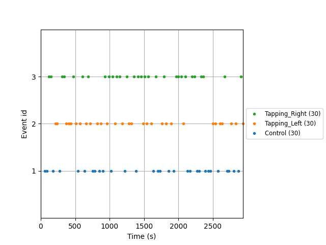
Next we examine the timing and order of events in this experiment. There are several options for how to view event information. The first option is to use MNE’s plot events command. Here each dot represents when an event started. We observe that the order of conditions was randomised and the time between events is also randomised.
events, event_dict = mne.events_from_annotations(raw_haemo, verbose=False)
mne.viz.plot_events(events, event_id=event_dict, sfreq=raw_haemo.info["sfreq"])
<Figure size 640x480 with 1 Axes>
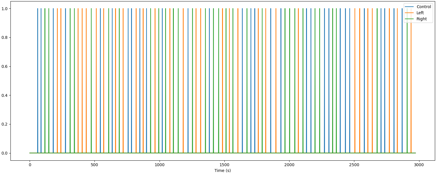
The previous plot did not illustrate the duration that an event lasted for. Alternatively, we can view the experiment using a boxcar plot, where the line is raised for the duration of the stimulus/condition.
s = mne_nirs.experimental_design.create_boxcar(raw_haemo)
fig, ax = plt.subplots(figsize=(15, 6), constrained_layout=True)
ax.plot(raw_haemo.times, s)
ax.legend(["Control", "Left", "Right"], loc="upper right")
ax.set_xlabel("Time (s)")
Used Annotations descriptions: ['Control', 'Tapping_Left', 'Tapping_Right']

Text(0.5, 18.167, 'Time (s)')
Create design matrix#
Next we create a model to fit our data to. The model consists of various components to model different things we assume contribute to the measured signal. We model the expected neural response for each experimental condition using the SPM haemodynamic response function (HRF) combined with the known stimulus event times and durations (as described above). We also include a cosine drift model with components up to the high pass parameter value. See the nilearn documentation for recommendations on setting these values. In short, they suggest “The cutoff period (1/high_pass) should be set as the longest period between two trials of the same condition multiplied by 2. For instance, if the longest period is 32s, the high_pass frequency shall be 1/64 Hz ~ 0.016 Hz”.
design_matrix = make_first_level_design_matrix(
    raw_haemo,
    drift_model="cosine",
    high_pass=0.005,  # Must be specified per experiment
    hrf_model="spm",
    stim_dur=5.0,
)
We also add the mean of the short channels to the design matrix. In theory these channels contain only systemic components, so including them in the design matrix allows us to estimate the neural component related to each experimental condition uncontaminated by systemic effects.
design_matrix["ShortHbO"] = np.mean(
    short_chs.copy().pick(picks="hbo").get_data(), axis=0
)

design_matrix["ShortHbR"] = np.mean(
    short_chs.copy().pick(picks="hbr").get_data(), axis=0
)
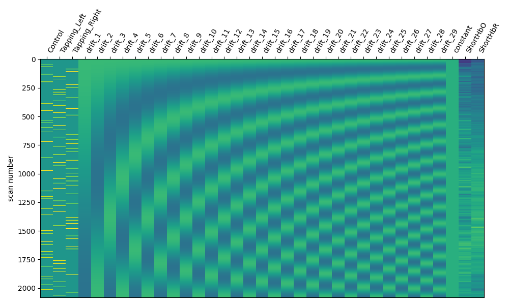
And we display a summary of the design matrix using standard Nilearn reporting functions. The first three columns represent the SPM HRF convolved with our stimulus event information. The next columns illustrate the drift and constant components. The last columns illustrate the short channel signals.
fig, ax1 = plt.subplots(figsize=(10, 6), constrained_layout=True)
fig = plot_design_matrix(design_matrix, ax=ax1)
Examine expected response#
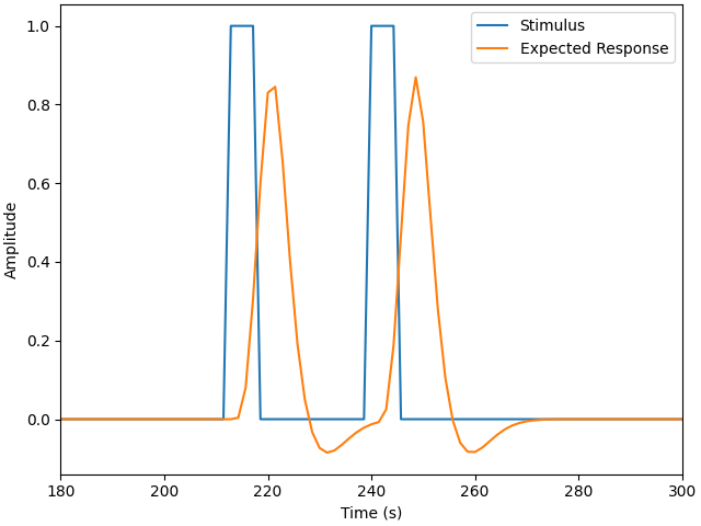
The matrices above can be a bit abstract as they encompase multiple conditions and regressors. Instead we can examine a single condition. Here we observe the boxcar function for a single condition, this illustrates when the stimulus was active. We also view the expected neural response using the HRF specified above, we observe that each time a stimulus is presented there is an expected brain response that lags the stimulus onset and consists of a large positive component followed by an undershoot.
In this example the second trigger (index 1) corresponds to the Tapping/Left
condition in the design matrix, so we plot those below. In your data the mapping
may be different, so you may need to alter either the s index or condition
name. Note however, that this is just for visualisation and does not affect
the results below.
fig, ax = plt.subplots(constrained_layout=True)
s = mne_nirs.experimental_design.create_boxcar(raw_intensity, stim_dur=5.0)
ax.plot(raw_intensity.times, s[:, 1])
ax.plot(design_matrix["Tapping_Left"])
ax.legend(["Stimulus", "Expected Response"])
ax.set(xlim=(180, 300), xlabel="Time (s)", ylabel="Amplitude")
Used Annotations descriptions: ['Control', 'Tapping_Left', 'Tapping_Right']

[(180.0, 300.0), Text(0.5, 18.167, 'Time (s)'), Text(18.167, 0.5, 'Amplitude')]
Fit GLM to subset of data and estimate response for each experimental condition#
We run a GLM fit for the data and experiment matrix. First we analyse just the first two channels which correspond to HbO and HbR of a single source detector pair.
data_subset = raw_haemo.copy().pick(picks=range(2))
glm_est = run_glm(data_subset, design_matrix)
This returns a GLM regression estimate for each channel. This data is stored in a dedicated type. You can view an overview of the estimates by addressing the variable:
GLM Results for 2 channels
As with other MNE types you can use the pick function. To query the mean square error of a single channel you would call.
Note: as we wish to retain both channels for further the analysis below, we operate on a copy to demonstrate this channel picking functionality.
glm_est.copy().pick("S1_D1 hbr")
GLM Results for 1 channels
Underlying the data for each channel is a standard Nilearn RegressionResults object object. These objects are rich with information that can be requested from the object, for example to determine the mean square error of the estimates for two channels you would call:
[3.6359501281260763e-11, 9.482010775760918e-12]
And we can chain the methods to quickly access required details. For example, to determine the MSE for channel S1 D1 for the hbr type you would call:
glm_est.copy().pick("S1_D1 hbr").MSE()
[9.482010775760918e-12]
Due to the richness of the objects we provide a function to extract commonly used information and put it in a convenient dataframe/table. Below this is demonstrated and then we just display the first 9 rows of the table which correspond to the 9 components of the design matrix for the first channel.
glm_est.to_dataframe().head(9)
We then display the results using the scatter plot function. Note that the control condition sits around zero and that the HbO is positive and larger than the HbR, this is to be expected. Further, we note that for this channel the response to tapping on the right hand is larger than the left. And the values are similar to what is seen in the epoching tutorial.
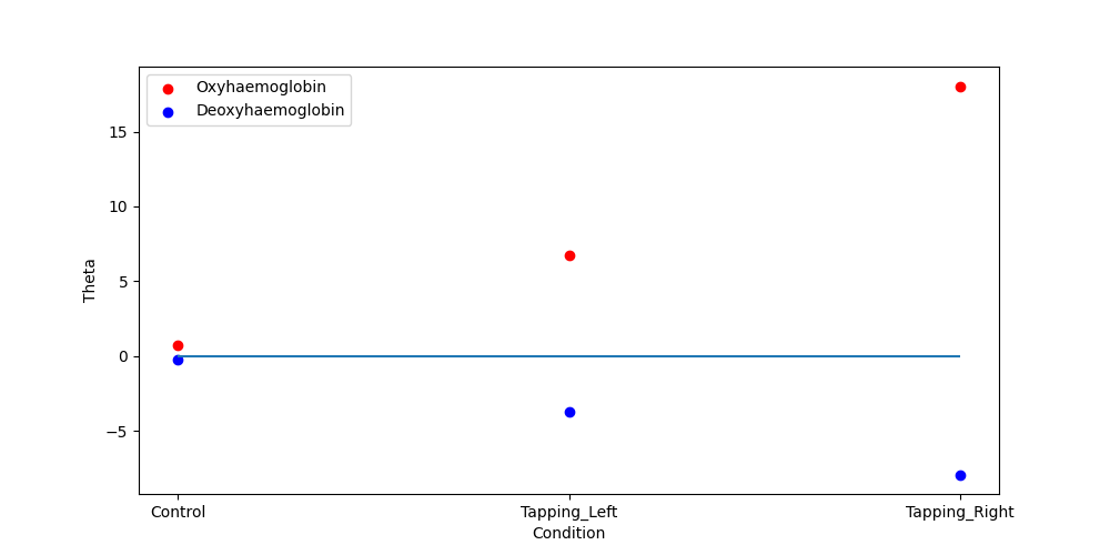
<AxesSubplot: xlabel='Condition', ylabel='Theta'>
Fit GLM to all data and view topographic distribution#
Lastly we can run the GLM analysis on all sensors and plot the result on a topomap. We see the same result as in the MNE tutorial, that activation is largest contralateral to the tapping side. Also note that HbR tends to be the negative of HbO as expected.
glm_est = run_glm(raw_haemo, design_matrix)
glm_est.plot_topo(conditions=["Tapping_Left", "Tapping_Right"])
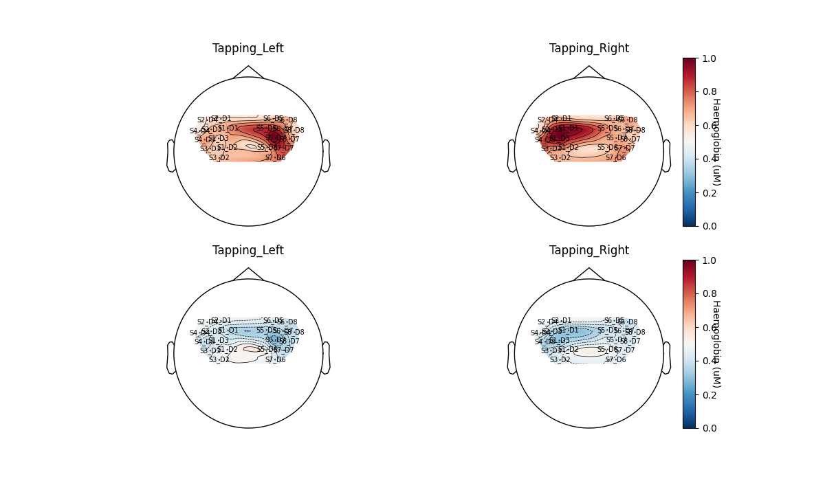
<Figure size 1200x700 with 6 Axes>
Note that the topographic visualisation is a high level representation of the underlying data. This visual representation fits a smoothed surface to the data and makes many assumptions including that the data is spatially smooth and that the sensors sufficiently cover the scalp surface. These assumptions can be violated with fNIRS due to the improved spatial sensitivity (relative to EEG) and typically low number of sensors that are unevenly distributed over the scalp. As such, researchers should understand the underlying data and ensure that the figure accurately reflects the effect of interest.
As an example of how the topoplot can be deceiving, we replot the Tapping/Right condition from above for each hemisphere separately. When both hemisphere are plotted together (left), the function smooths the large space between sensors, making the activity on the left hemisphere smear towards the center and appear larger than the underlying data shows. When each hemisphere is plotted independently (right) it becomes immediately apparent that the data does not indicate that activity spreads across the center of the head.
fig, axes = plt.subplots(
    nrows=1, ncols=2, figsize=(10, 6), gridspec_kw=dict(width_ratios=[0.92, 1])
)

glm_hbo = glm_est.copy().pick(picks="hbo")
conditions = ["Tapping_Right"]

glm_hbo.plot_topo(axes=axes[0], colorbar=False, conditions=conditions)

glm_hbo.copy().pick(picks=range(10)).plot_topo(
    conditions=conditions, axes=axes[1], colorbar=False, vlim=(-16, 16)
)
glm_hbo.copy().pick(picks=range(10, 20)).plot_topo(
    conditions=conditions, axes=axes[1], colorbar=False, vlim=(-16, 16)
)

axes[0].set_title("Smoothed across hemispheres")
axes[1].set_title("Hemispheres plotted independently")
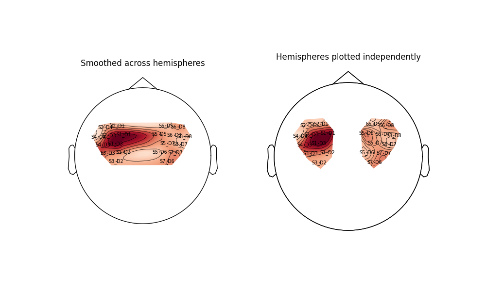
Text(0.5, 1.0, 'Hemispheres plotted independently')
Another way to view the data is to project the GLM estimates to the nearest cortical surface
glm_est.copy().surface_projection(
    condition="Tapping_Right", view="dorsal", chroma="hbo"
)
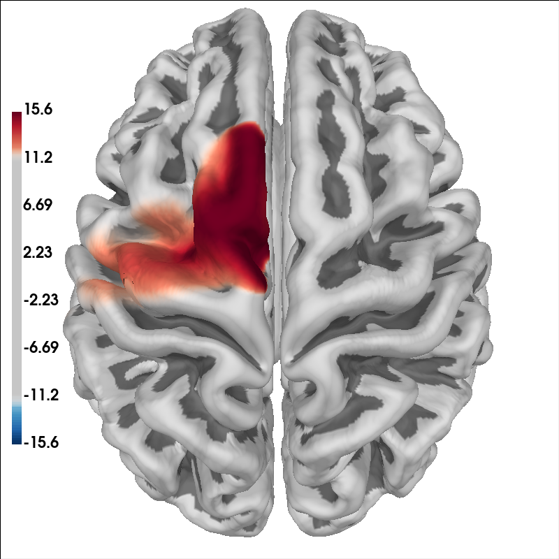
<mne.viz._brain._brain.Brain object at 0x7fdb2873f580>
Analyse regions of interest#
Or alternatively we can summarise the responses across regions of interest for each condition. And you can plot it with your favorite software. Region of interest analysis can be more robust than single channel analysis. The fOLD toolbox can be used to assist in the design of ROIs. And consideration should be paid to ensure optimal size ROIs are selected.
left = [[1, 1], [1, 2], [1, 3], [2, 1], [2, 3], [2, 4], [3, 2], [3, 3], [4, 3], [4, 4]]
right = [[5, 5], [5, 6], [5, 7], [6, 5], [6, 7], [6, 8], [7, 6], [7, 7], [8, 7], [8, 8]]

groups = dict(
    Left_ROI=picks_pair_to_idx(raw_haemo, left),
    Right_ROI=picks_pair_to_idx(raw_haemo, right),
)

conditions = ["Control", "Tapping_Left", "Tapping_Right"]

df = glm_est.to_dataframe_region_of_interest(groups, conditions)
As with the single channel results above, this is placed in a tidy dataframe which contains conveniently extracted information, but now for the region of interest.
Compute contrasts#
We can also define a contrast as described in Nilearn docs and plot it. Here we contrast the response to tapping on the left hand with the response from tapping on the right hand.
contrast_matrix = np.eye(design_matrix.shape[1])
basic_conts = dict(
    [(column, contrast_matrix[i]) for i, column in enumerate(design_matrix.columns)]
)
contrast_LvR = basic_conts["Tapping_Left"] - basic_conts["Tapping_Right"]

contrast = glm_est.compute_contrast(contrast_LvR)
contrast.plot_topo()
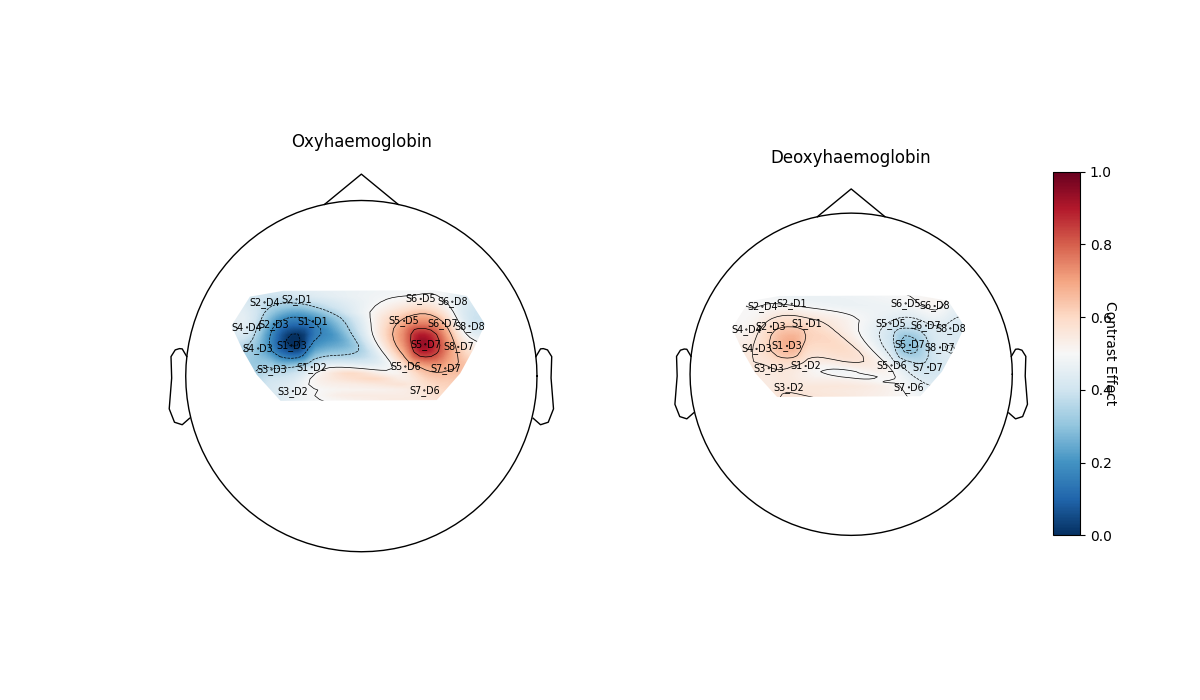
<Figure size 1200x700 with 3 Axes>
Export Results#
Here we export the data in a tidy pandas data frame. We export the GLM results for every channel and condition. Data is exported in long format by default. However, a helper function is also provided to convert the long data to wide format. The long to wide conversion also adds some additional derived data, such as if a significant response (p<0.05) was observed, which sensor and detector is in the channel, which chroma, etc.
Determine true and false positive rates#
We can query the exported data frames to determine the true and false positive rates. Note: optodes cover a greater region than just the motor cortex, so we dont expect 100% of channels to detect responses to the tapping, but we do expect 5% or less for the false positive rate.
(
    df.query('Condition in ["Control", "Tapping_Left", "Tapping_Right"]')
    .drop(["df", "mse", "p_value", "t"], axis=1)
    .groupby(["Condition", "Chroma", "ch_name"])
    .agg(["mean"])
)
Total running time of the script: (0 minutes 13.077 seconds)
Estimated memory usage: 664 MB