Utilising Anatomical Information

This example demonstrates how you can utilise anatomical and sensor position information in your analysis pipeline. This information can be used to verify measurement/analysis and also improve analysis accuracy [1].

This example demonstrates how to plot your data on a 3D brain and overlay the sensor locations and regions of interest.

This tutorial glosses over the processing details, see the GLM tutorial for details on the preprocessing.

# sphinx_gallery_thumbnail_number = 5

# Authors: Robert Luke <mail@robertluke.net>
#
# License: BSD (3-clause)

import numpy as np
import pandas as pd

import mne
from mne.preprocessing.nirs import optical_density, beer_lambert_law

import statsmodels.formula.api as smf

from mne_bids import BIDSPath, read_raw_bids, get_entity_vals
import mne_nirs

from mne_nirs.experimental_design import make_first_level_design_matrix
from mne_nirs.statistics import run_glm, statsmodels_to_results
from mne_nirs.channels import get_long_channels, get_short_channels
from mne_nirs.io.fold import fold_landmark_specificity
from mne_nirs.visualisation import plot_nirs_source_detector, plot_glm_surface_projection
from mne_nirs.datasets import fnirs_motor_group

Download example data

First, the data required data for this tutorial is downloaded.

Download example fNIRS data

Download the audio_or_visual_speech dataset and load the first measurement.

root = mne_nirs.datasets.audio_or_visual_speech.data_path()
dataset = BIDSPath(root=root, suffix="nirs", extension=".snirf", subject="04",
                   task="AudioVisualBroadVsRestricted", datatype="nirs", session="01")
raw = mne.io.read_raw_snirf(dataset.fpath)
raw.annotations.rename({'1.0': 'Audio',
                        '2.0': 'Video',
                        '3.0': 'Control',
                        '15.0': 'Ends'})

<Annotations | 48 segments: Audio (18), Control (10), Ends (2), Video (18)>

Download annotation information

Download the HCP-MMP parcellation.

# Download anatomical locations
subjects_dir = str(mne.datasets.sample.data_path()) + '/subjects'
mne.datasets.fetch_hcp_mmp_parcellation(subjects_dir=subjects_dir, accept=True)
labels = mne.read_labels_from_annot('fsaverage', 'HCPMMP1', 'lh', subjects_dir=subjects_dir)
labels_combined = mne.read_labels_from_annot('fsaverage', 'HCPMMP1_combined', 'lh', subjects_dir=subjects_dir)

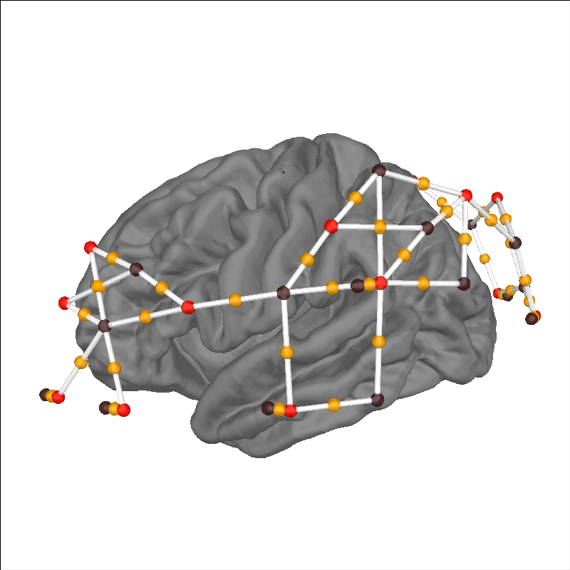
Verify placement of sensors

The first thing we can do is plot the location of the optodes and channels over an average brain surface to verify the data, specifically the 3D coordinates, have been loaded correctly. The sources are represented as red dots, the detectors are represented as black dots, the whit lines represent source-detector pairs, and the orange dots represent channel locations. In this example we can see channels over the left inferior frontal gyrus, auditory cortex, planum temporale, and occipital lobe.

brain = mne.viz.Brain('fsaverage', subjects_dir=subjects_dir, background='w', cortex='0.5')
brain.add_sensors(raw.info, trans='fsaverage', fnirs=['channels', 'pairs', 'sources', 'detectors'])
brain.show_view(azimuth=180, elevation=80, distance=450)

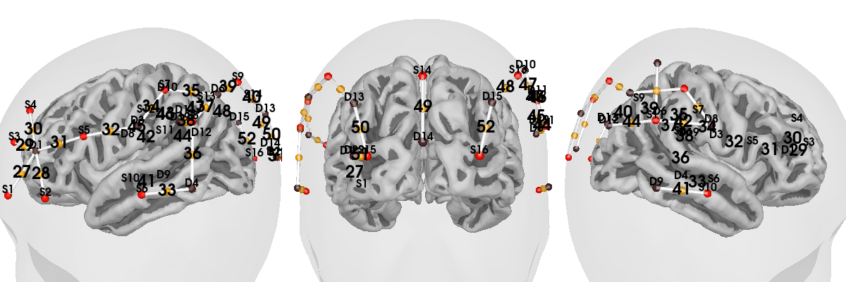
Plot sensor channel numbers

Often for publications and sanity checking, it’s convenient to create an image showing the channel numbers along with the (typically) 10-20 location in the correct locations in a 3D view. The function mne_nirs.visualisation.plot_3d_montage() gives us this once we specify which views to use to show each channel pair:

view_map = {
    'left-lat': np.r_[np.arange(1, 27), 28],
    'caudal': np.r_[27, np.arange(43, 53)],
    'right-lat': np.r_[np.arange(29, 43), 44],
}

fig_montage = mne_nirs.visualisation.plot_3d_montage(
    raw.info, view_map=view_map, subjects_dir=subjects_dir)

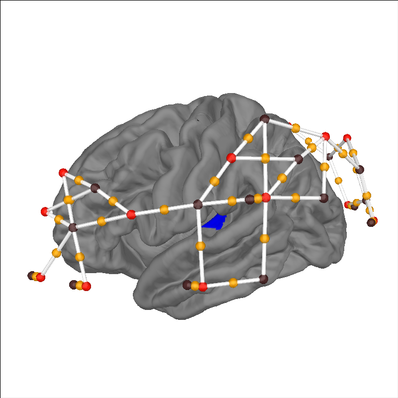
Plot sensor channels and anatomical region of interest

Once the data has been loaded we can highlight anatomical regions of interest to ensure that the sensors are appropriately placed to measure from the relevant brain structures. In this example we highlight the primary auditory cortex in blue, and we can see that a number of channels are placed over this structure.

brain = mne.viz.Brain('fsaverage', subjects_dir=subjects_dir, background='w', cortex='0.5')
brain.add_sensors(raw.info, trans='fsaverage', fnirs=['channels', 'pairs', 'sources', 'detectors'])

aud_label = [label for label in labels if label.name == 'L_A1_ROI-lh'][0]
brain.add_label(aud_label, borders=False, color='blue')
brain.show_view(azimuth=180, elevation=80, distance=450)

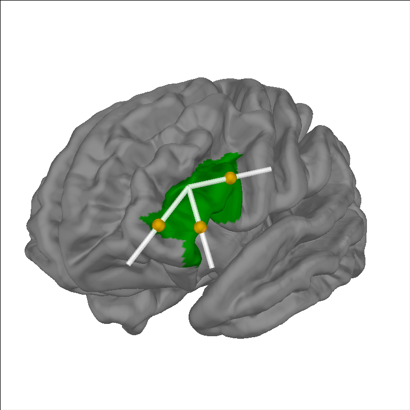
Plot channels sensitive to anatomical region of interest

fOLD Toolbox

You should use the fOLD toolbox to pick your optode locations when designing your experiment. The tool is very intuitive and easy to use. Be sure to cite the authors if you use their tool or data:

Morais, Guilherme Augusto Zimeo, Joana Bisol Balardin, and João Ricardo Sato. “fNIRS optodes’ location decider (fOLD): a toolbox for probe arrangement guided by brain regions-of-interest.” Scientific reports 8.1 (2018): 1-11.

Rather than simply eye balling the sensor and ROIs of interest, we can quantify the specificity of each channel to the anatomical region of interest and select channels that are sufficiently sensitive for further analysis. In this example we highlight the left inferior frontal gyrus (IFG) and use data from the fOLD toolbox [2]. To see more details about how to use the fOLD data see this tutorial.

# Return specificity of each channel to the Left IFG
specificity = fold_landmark_specificity(raw, 'L IFG (p. Triangularis)')

# Retain only channels with specificity to left IFG of greater than 50%
raw_IFG = raw.copy().pick(picks=np.where(specificity > 50)[0])

brain = mne.viz.Brain('fsaverage', subjects_dir=subjects_dir, background='w', cortex='0.5')
brain.add_sensors(raw_IFG.info, trans='fsaverage', fnirs=['channels', 'pairs'])

ifg_label = [label for label in labels_combined if label.name == 'Inferior Frontal Cortex-lh'][0]
brain.add_label(ifg_label, borders=False, color='green')

brain.show_view(azimuth=140, elevation=95, distance=360)

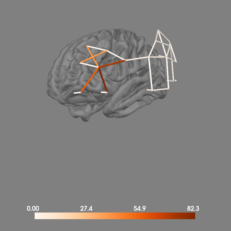
Alternatively, we can retain all channels and visualise the specificity of each channel the ROI by encoding the specificty in the color of the line between each source and detector. In this example we see that several channels have substantial specificity to the region of interest.

Note: this function currently doesn’t support the new MNE brain API, so does not allow the same behaviour as above (adding sensors, highlighting ROIs etc). It should be updated in the near future.

fig = plot_nirs_source_detector(specificity, raw.info, surfaces='brain',
                                subject='fsaverage', subjects_dir=subjects_dir, trans='fsaverage')
mne.viz.set_3d_view(fig, azimuth=140, elevation=95)

Anatomically informed weighting in region of interest analysis

As observed above, some channels have greater specificity to the desired brain region than other channels. Thus, when doing a region of interest analysis you may wish to give extra weight to channels with greater sensitivity to the desired ROI. This can be done by manually specifying the weights used in the region of interest function call. The details of the GLM analysis will not be described here, instead view the fNIRS GLM tutorial. Instead, comments are provided for the weighted region of interest function call.

# Basic pipeline, simplified for example
raw_od = optical_density(raw)
raw_haemo = beer_lambert_law(raw_od)
raw_haemo.resample(0.3).pick("hbo")  # Speed increase for web server
sht_chans = get_short_channels(raw_haemo)
raw_haemo = get_long_channels(raw_haemo)
design_matrix = make_first_level_design_matrix(raw_haemo, stim_dur=13.0)
design_matrix["ShortHbO"] = np.mean(sht_chans.copy().pick(picks="hbo").get_data(), axis=0)
glm_est = run_glm(raw_haemo, design_matrix)

# First we create a dictionary for each region of interest.
# Here we include all channels in each ROI, as we will later be applying
# weights based on their specificity to the brain regions of interest.
rois = dict()
rois["Audio_weighted"] = range(len(glm_est.ch_names))
rois["Visual_weighted"] = range(len(glm_est.ch_names))

# Next we compute the specificity for each channel to the auditory and visual cortex.
spec_aud = fold_landmark_specificity(raw_haemo, '42 - Primary and Auditory Association Cortex', atlas="Brodmann")
spec_vis = fold_landmark_specificity(raw_haemo, '17 - Primary Visual Cortex (V1)', atlas="Brodmann")

# Next we create a dictionary to store the weights for each channel in the ROI.
# The weights will be the specificity to the ROI.
# The keys and length of each dictionary entry must match the ROI dictionary.
weights = dict()
weights["Audio_weighted"] = spec_aud
weights["Visual_weighted"] = spec_vis

# Finally we compute region of interest results using the weights specified above
out = glm_est.to_dataframe_region_of_interest(rois, ["Video", "Control"], weighted=weights)
out["Significant"] = out["p"] < 0.05
out

	ROI	Condition	Chroma	theta	se	t	dfe	p	Weighted	Significant
0	Audio_weighted	Video	hbo	-1.116166e-08	0.027915	-0.399851	43	0.691246	Custom	False
1	Visual_weighted	Video	hbo	9.230472e-08	0.025380	3.636926	43	0.000734	Custom	True
0	Audio_weighted	Control	hbo	-4.551715e-10	0.036879	-0.012342	43	0.990210	Custom	False
1	Visual_weighted	Control	hbo	-1.807595e-08	0.033537	-0.538982	43	0.592679	Custom	False

In the table above we observe that the response to the visual condition is only present in the visual region of interest. You can use this technique to load any custom weighting, including weights exported from other software.

Preprocess fNIRS data

We can also use the 3D information to project the results on to the cortical surface. First, we process the fNIRS data. This is a duplication of the GLM tutorial analysis. The details will not be described here, instead view the fNIRS GLM tutorial.

def individual_analysis(bids_path, ID):

    raw_intensity = read_raw_bids(bids_path=bids_path, verbose=False)
    raw_intensity.annotations.delete(raw_intensity.annotations.description == '15.0')
     # sanitize event names
    raw_intensity.annotations.description[:] = [
        d.replace('/', '_') for d in raw_intensity.annotations.description]

    # Convert signal to haemoglobin and resample
    raw_od = optical_density(raw_intensity)
    raw_haemo = beer_lambert_law(raw_od, ppf=0.1)
    raw_haemo.resample(0.3)

    # Cut out just the short channels for creating a GLM repressor
    sht_chans = get_short_channels(raw_haemo)
    raw_haemo = get_long_channels(raw_haemo)

    # Create a design matrix
    design_matrix = make_first_level_design_matrix(raw_haemo, stim_dur=5.0)

    # Append short channels mean to design matrix
    design_matrix["ShortHbO"] = np.mean(sht_chans.copy().pick(picks="hbo").get_data(), axis=0)
    design_matrix["ShortHbR"] = np.mean(sht_chans.copy().pick(picks="hbr").get_data(), axis=0)

    # Run GLM
    glm_est = run_glm(raw_haemo, design_matrix)

    # Extract channel metrics
    cha = glm_est.to_dataframe()

    # Add the participant ID to the dataframes
    cha["ID"] = ID

    # Convert to uM for nicer plotting below.
    cha["theta"] = [t * 1.e6 for t in cha["theta"]]

    return raw_haemo, cha


# Get dataset details
root = fnirs_motor_group.data_path()
dataset = BIDSPath(root=root, task="tapping",
                   datatype="nirs", suffix="nirs", extension=".snirf")
subjects = get_entity_vals(root, 'subject')

df_cha = pd.DataFrame()  # To store channel level results
for sub in subjects:  # Loop from first to fifth subject

    # Create path to file based on experiment info
    bids_path = dataset.update(subject=sub)

    # Analyse data and return both ROI and channel results
    raw_haemo, channel = individual_analysis(bids_path, sub)

    # Append individual results to all participants
    df_cha = pd.concat([df_cha, channel], ignore_index=True)

ch_summary = df_cha.query("Condition in ['Tapping_Right']")
assert len(ch_summary)
ch_summary = ch_summary.query("Chroma in ['hbo']")
ch_model = smf.mixedlm("theta ~ -1 + ch_name", ch_summary,
                       groups=ch_summary["ID"]).fit(method='nm')
model_df = statsmodels_to_results(ch_model, order=raw_haemo.copy().pick("hbo").ch_names)

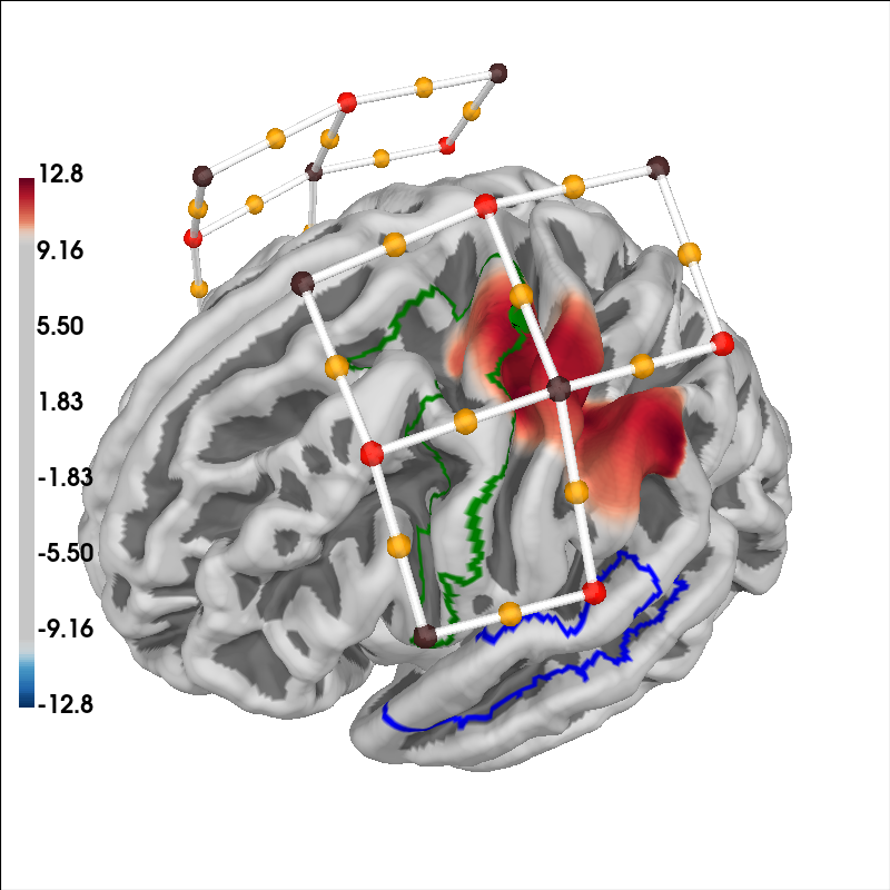
Plot surface projection of GLM results

Finally, we can project the GLM results from each channel to the nearest cortical surface and overlay the sensor positions and two different regions of interest. In this example we also highlight the premotor cortex and auditory association cortex in green and blue respectively.

# Plot the projection and sensor locations
brain = plot_glm_surface_projection(raw_haemo.copy().pick("hbo"), model_df, colorbar=True)
brain.add_sensors(raw_haemo.info, trans='fsaverage', fnirs=['channels', 'pairs', 'sources', 'detectors'])

# mark the premotor cortex in green
aud_label = [label for label in labels_combined if label.name == 'Premotor Cortex-lh'][0]
brain.add_label(aud_label, borders=True, color='green')

# mark the auditory association cortex in blue
aud_label = [label for label in labels_combined if label.name == 'Auditory Association Cortex-lh'][0]
brain.add_label(aud_label, borders=True, color='blue')

brain.show_view(azimuth=160, elevation=60, distance=400)

Bibliography

[1]

Sergio Luiz Novi, Edwin Johan Forero, Jose Angel Ivan Rubianes Silva, Nicolas Gabriel SR de Souza, Giovani Grisotti Martins, Andres Quiroga, Shin-Ting Wu, and Rickson C Mesquita. Integration of spatial information increases reproducibility in functional near-infrared spectroscopy. Frontiers in neuroscience, 2020. doi:10.3389/fnins.2020.00746.

[2]

Guilherme Augusto Zimeo Morais, Joana Bisol Balardin, and João Ricardo Sato. Fnirs optodes’ location decider (fold): a toolbox for probe arrangement guided by brain regions-of-interest. Scientific reports, 8(1):1–11, 2018.

Estimated memory usage: 26 MB