Note
Go to the end to download the full example code. or to run this example in your browser via Binder
Group Level Waveform Analysis#
This is an example of a group-level waveform-based functional near-infrared spectroscopy (fNIRS) analysis in MNE-NIRS.
Individual-level analysis of this data is described in the MNE-NIRS fNIRS waveform tutorial and the MNE-NIRS fNIRS GLM tutorial. As such, this example will skim over the individual-level details and focus on the group-level aspects of analysis. Here we describe how to process multiple measurements and how to summarise group-level effects either by visual presentation of the results or with summary statistics.
The data used in this example is available at this location. The data was collected from a finger tapping experiment that is briefly described below. The dataset contains 5 participants. The example dataset is in BIDS format and therefore already contains information about triggers, condition names, etc.
Note
This tutorial uses data stored using the BIDS format [1].
MNE-Python allows you to process fNIRS data that is not in BIDS format.
Simply modify the read_raw_ function to match your data type.
See data importing tutorial to learn how
to use your data with MNE-Python.
Note
Optodes were placed over the motor cortex using the standard NIRx motor montage with 8 short channels added (see their web page for details). To view the sensor locations run raw_intensity.plot_sensors(). A 5 sec sound was presented in either the left or right ear to indicate which hand the participant should tap. Participants tapped their thumb to their fingers for the entire 5 sec. Conditions were presented in a random order with a randomised inter- stimulus interval.
# sphinx_gallery_thumbnail_number = 2

# Authors: Robert Luke <mail@robertluke.net>
#
# License: BSD (3-clause)

# Import common libraries
from collections import defaultdict
from copy import deepcopy
from itertools import compress
from pprint import pprint

# Import Plotting Library
import matplotlib.pyplot as plt
import pandas as pd
import seaborn as sns

# Import StatsModels
import statsmodels.formula.api as smf
from mne import Epochs, events_from_annotations, set_log_level
from mne.preprocessing.nirs import (
    beer_lambert_law,
    optical_density,
    scalp_coupling_index,
    temporal_derivative_distribution_repair,
)

# Import MNE processing
from mne.viz import plot_compare_evokeds

# Import MNE-BIDS processing
from mne_bids import BIDSPath, read_raw_bids

# Import MNE-NIRS processing
from mne_nirs.channels import get_long_channels, picks_pair_to_idx
from mne_nirs.datasets import fnirs_motor_group
from mne_nirs.signal_enhancement import enhance_negative_correlation

# Set general parameters
set_log_level("WARNING")  # Don't show info, as it is repetitive for many subjects
Define individual analysis#
First, we define the analysis that will be applied to each participant file. This is the same waveform analysis as described in the individual waveform tutorial and artifact correction tutorial. As such, this example will skim over the individual-level details.
def individual_analysis(bids_path):
    # Read data with annotations in BIDS format
    raw_intensity = read_raw_bids(bids_path=bids_path, verbose=False)
    raw_intensity = get_long_channels(raw_intensity, min_dist=0.01)

    # Convert signal to optical density and determine bad channels
    raw_od = optical_density(raw_intensity)
    sci = scalp_coupling_index(raw_od, h_freq=1.35, h_trans_bandwidth=0.1)
    raw_od.info["bads"] = list(compress(raw_od.ch_names, sci < 0.5))
    raw_od.interpolate_bads()

    # Downsample and apply signal cleaning techniques
    raw_od.resample(0.8)
    raw_od = temporal_derivative_distribution_repair(raw_od)

    # Convert to haemoglobin and filter
    raw_haemo = beer_lambert_law(raw_od, ppf=0.1)
    raw_haemo = raw_haemo.filter(
        0.02, 0.3, h_trans_bandwidth=0.1, l_trans_bandwidth=0.01, verbose=False
    )

    # Apply further data cleaning techniques and extract epochs
    raw_haemo = enhance_negative_correlation(raw_haemo)
    # Extract events but ignore those with
    # the word Ends (i.e. drop ExperimentEnds events)
    events, event_dict = events_from_annotations(
        raw_haemo, verbose=False, regexp="^(?![Ends]).*$"
    )
    epochs = Epochs(
        raw_haemo,
        events,
        event_id=event_dict,
        tmin=-5,
        tmax=20,
        reject=dict(hbo=200e-6),
        reject_by_annotation=True,
        proj=True,
        baseline=(None, 0),
        detrend=0,
        preload=True,
        verbose=False,
    )

    return raw_haemo, epochs
Run analysis on all data#
Next, we loop through the five participants’ measurements and run the individual analysis on each. For each individual, the function returns the raw data and an epoch structure. The epoch structure is then averaged to obtain an evoked response from each participant. The individual-evoked data is stored in a dictionary (all_evokeds) for each condition.
all_evokeds = defaultdict(list)

for sub in range(1, 6):  # Loop from first to fifth subject
    # Create path to file based on experiment info
    bids_path = BIDSPath(
        subject="%02d" % sub,
        task="tapping",
        datatype="nirs",
        root=fnirs_motor_group.data_path(),
        suffix="nirs",
        extension=".snirf",
    )

    # Analyse data and return both ROI and channel results
    raw_haemo, epochs = individual_analysis(bids_path)

    # Save individual-evoked participant data along with others in all_evokeds
    for cidx, condition in enumerate(epochs.event_id):
        all_evokeds[condition].append(epochs[condition].average())
/home/circleci/project/examples/general/plot_16_waveform_group.py:136: RuntimeWarning: No bad channels to interpolate. Doing nothing...
  raw_od.interpolate_bads()
/home/circleci/project/examples/general/plot_16_waveform_group.py:136: RuntimeWarning: No bad channels to interpolate. Doing nothing...
  raw_od.interpolate_bads()
The end result is a dictionary that is indexed per condition, with each item in the dictionary being a list of evoked responses. See below that for each condition we have obtained a MNE evoked type that is generated from the average of all 30 trials and epoched from -5 to 20 seconds.
defaultdict(<class 'list'>,
            {'15.0': [<Evoked | '15.0' (average, N=1), -5 – 20 s, baseline -5 – 0 s, 40 ch, ~63 kB>,
                      <Evoked | '15.0' (average, N=2), -5 – 20 s, baseline -5 – 0 s, 40 ch, ~63 kB>,
                      <Evoked | '15.0' (average, N=1), -5 – 20 s, baseline -5 – 0 s, 40 ch, ~63 kB>,
                      <Evoked | '15.0' (average, N=2), -5 – 20 s, baseline -5 – 0 s, 40 ch, ~63 kB>,
                      <Evoked | '15.0' (average, N=1), -5 – 20 s, baseline -5 – 0 s, 40 ch, ~63 kB>],
             'Control': [<Evoked | 'Control' (average, N=30), -5 – 20 s, baseline -5 – 0 s, 40 ch, ~63 kB>,
                         <Evoked | 'Control' (average, N=30), -5 – 20 s, baseline -5 – 0 s, 40 ch, ~63 kB>,
                         <Evoked | 'Control' (average, N=30), -5 – 20 s, baseline -5 – 0 s, 40 ch, ~63 kB>,
                         <Evoked | 'Control' (average, N=30), -5 – 20 s, baseline -5 – 0 s, 40 ch, ~63 kB>,
                         <Evoked | 'Control' (average, N=30), -5 – 20 s, baseline -5 – 0 s, 40 ch, ~63 kB>],
             'Tapping/Left': [<Evoked | 'Tapping/Left' (average, N=30), -5 – 20 s, baseline -5 – 0 s, 40 ch, ~63 kB>,
                              <Evoked | 'Tapping/Left' (average, N=30), -5 – 20 s, baseline -5 – 0 s, 40 ch, ~63 kB>,
                              <Evoked | 'Tapping/Left' (average, N=30), -5 – 20 s, baseline -5 – 0 s, 40 ch, ~63 kB>,
                              <Evoked | 'Tapping/Left' (average, N=30), -5 – 20 s, baseline -5 – 0 s, 40 ch, ~63 kB>,
                              <Evoked | 'Tapping/Left' (average, N=30), -5 – 20 s, baseline -5 – 0 s, 40 ch, ~63 kB>],
             'Tapping/Right': [<Evoked | 'Tapping/Right' (average, N=30), -5 – 20 s, baseline -5 – 0 s, 40 ch, ~63 kB>,
                               <Evoked | 'Tapping/Right' (average, N=30), -5 – 20 s, baseline -5 – 0 s, 40 ch, ~63 kB>,
                               <Evoked | 'Tapping/Right' (average, N=30), -5 – 20 s, baseline -5 – 0 s, 40 ch, ~63 kB>,
                               <Evoked | 'Tapping/Right' (average, N=30), -5 – 20 s, baseline -5 – 0 s, 40 ch, ~63 kB>,
                               <Evoked | 'Tapping/Right' (average, N=30), -5 – 20 s, baseline -5 – 0 s, 40 ch, ~63 kB>]})
View average waveform#
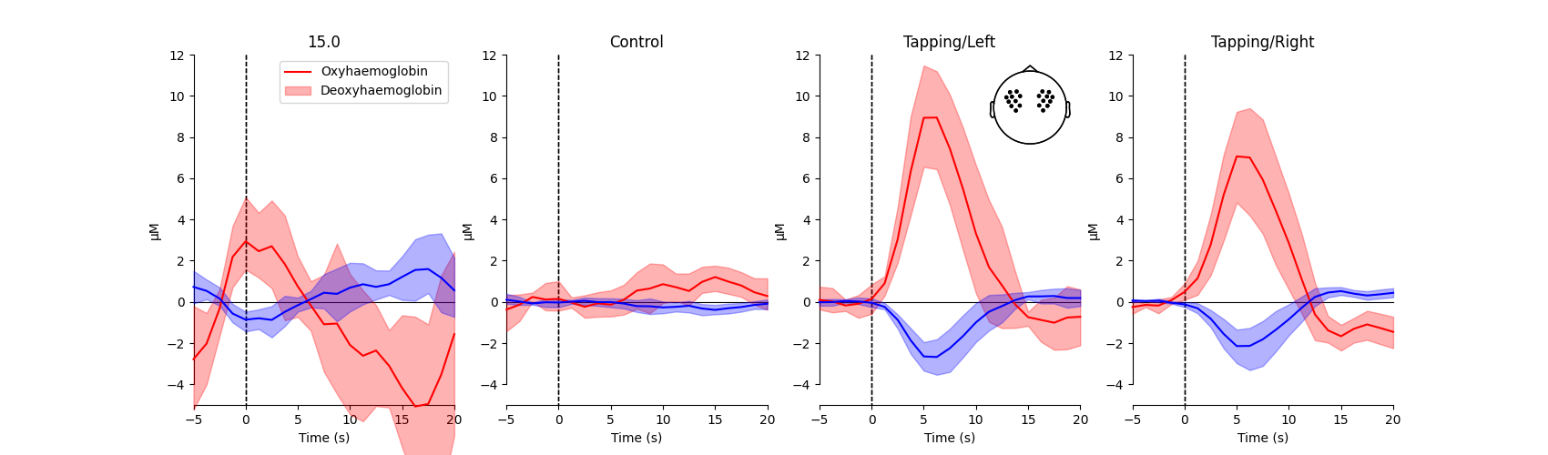
Next, a grand average epoch waveform is generated for each condition. This is generated using all of the standard (long) fNIRS channels, as illustrated by the head inset in the top right corner of the figure.
# Specify the figure size and limits per chromophore
fig, axes = plt.subplots(nrows=1, ncols=len(all_evokeds), figsize=(17, 5))
lims = dict(hbo=[-5, 12], hbr=[-5, 12])

for pick, color in zip(["hbo", "hbr"], ["r", "b"]):
    for idx, evoked in enumerate(all_evokeds):
        plot_compare_evokeds(
            {evoked: all_evokeds[evoked]},
            combine="mean",
            picks=pick,
            axes=axes[idx],
            show=False,
            colors=[color],
            legend=False,
            ylim=lims,
            ci=0.95,
            show_sensors=idx == 2,
        )
        axes[idx].set_title(f"{evoked}")
axes[0].legend(["Oxyhaemoglobin", "Deoxyhaemoglobin"])
<matplotlib.legend.Legend object at 0x7fdb244ffc70>
From this figure we observe that the response to the tapping condition with the right hand appears larger than when no tapping occurred in the control condition (similar for when tapping occurred with the left hand). We test if this is the case in the analysis below.
Generate regions of interest#
Here we specify two regions of interest (ROIs) by listing the source-detector pairs of interest and then determining which channels these correspond to within the raw data structure. The channel indices are stored in a dictionary for access below. The fOLD toolbox can be used to assist in the design of ROIs. And consideration should be paid to ensure optimal size ROIs are selected.
In this example, two ROIs are generated. One for the left motor cortex and one for the right motor cortex. These are called Left_Hemisphere and Right_Hemisphere and are stored in the rois dictionary.
# Specify channel pairs for each ROI
left = [[4, 3], [1, 3], [3, 3], [1, 2], [2, 3], [1, 1]]
right = [[8, 7], [5, 7], [7, 7], [5, 6], [6, 7], [5, 5]]

# Then generate the correct indices for each pair and store in dictionary
rois = dict(
    Left_Hemisphere=picks_pair_to_idx(raw_haemo, left),
    Right_Hemisphere=picks_pair_to_idx(raw_haemo, right),
)

pprint(rois)
{'Left_Hemisphere': [16, 17, 4, 5, 14, 15, 2, 3, 8, 9, 0, 1],
 'Right_Hemisphere': [36, 37, 24, 25, 34, 35, 22, 23, 28, 29, 20, 21]}
Create average waveform per ROI#
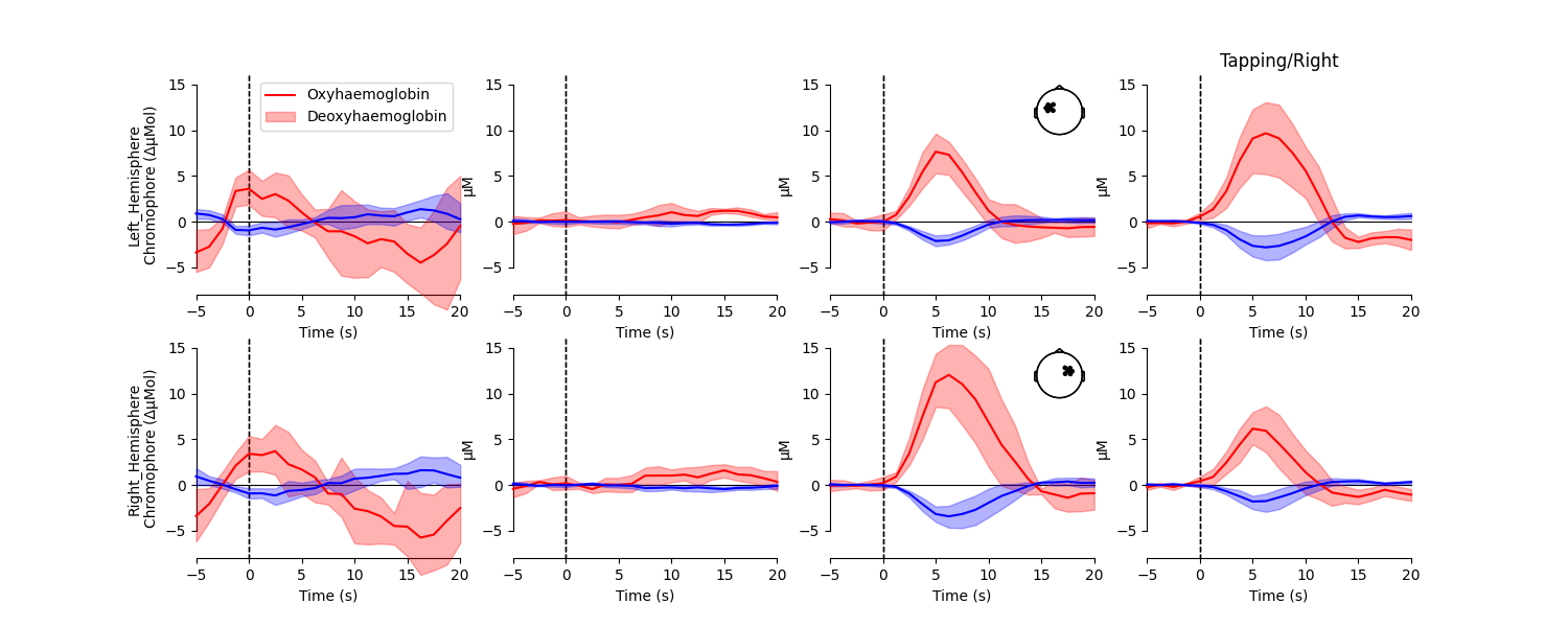
Next, an average waveform is generated per condition per region of interest. This allows the researcher to view the responses elicited in different regions of the brain for each condition.
# Specify the figure size and limits per chromophore.
fig, axes = plt.subplots(nrows=len(rois), ncols=len(all_evokeds), figsize=(15, 6))
lims = dict(hbo=[-8, 16], hbr=[-8, 16])

for pick, color in zip(["hbo", "hbr"], ["r", "b"]):
    for ridx, roi in enumerate(rois):
        for cidx, evoked in enumerate(all_evokeds):
            if pick == "hbr":
                picks = rois[roi][1::2]  # Select only the hbr channels
            else:
                picks = rois[roi][0::2]  # Select only the hbo channels

            plot_compare_evokeds(
                {evoked: all_evokeds[evoked]},
                combine="mean",
                picks=picks,
                axes=axes[ridx, cidx],
                show=False,
                colors=[color],
                legend=False,
                ylim=lims,
                ci=0.95,
                show_sensors=cidx == 2,
            )
            axes[ridx, cidx].set_title("")
        axes[0, cidx].set_title(f"{evoked}")
        axes[ridx, 0].set_ylabel(f"{roi}\nChromophore (ΔμMol)")
axes[0, 0].legend(["Oxyhaemoglobin", "Deoxyhaemoglobin"])
<matplotlib.legend.Legend object at 0x7fdb244ffa00>
From this figure we observe that the response to tapping appears largest in the brain region that is contralateral to the hand that is tapping. We test if this is the case in the analysis below.
Extract evoked amplitude#
The waveforms above provide a qualitative overview of the data. It is also useful to perform a quantitative analysis based on the relevant features in the dataset. Here we extract the average value of the waveform between 5 and 7 seconds for each subject, condition, region of interest, and chromophore. The data is then stored in a dataframe, which is saved to a csv file for easy analysis in any statistical analysis software. We also demonstrate two example analyses on these values below.
df = pd.DataFrame(columns=["ID", "ROI", "Chroma", "Condition", "Value"])

for idx, evoked in enumerate(all_evokeds):
    subj_id = 0
    for subj_data in all_evokeds[evoked]:
        subj_id += 1
        for roi in rois:
            for chroma in ["hbo", "hbr"]:
                data = deepcopy(subj_data).pick(picks=rois[roi]).pick(chroma)
                value = data.crop(tmin=5.0, tmax=7.0).data.mean() * 1.0e6

                # Append metadata and extracted feature to dataframe
                this_df = pd.DataFrame(
                    {
                        "ID": subj_id,
                        "ROI": roi,
                        "Chroma": chroma,
                        "Condition": evoked,
                        "Value": value,
                    },
                    index=[0],
                )
                df = pd.concat([df, this_df], ignore_index=True)
df.reset_index(inplace=True, drop=True)
df["Value"] = pd.to_numeric(df["Value"])  # some Pandas have this as object

# You can export the dataframe for analysis in your favorite stats program
df.to_csv("stats-export.csv")

# Print out the first entries in the dataframe
df.head()
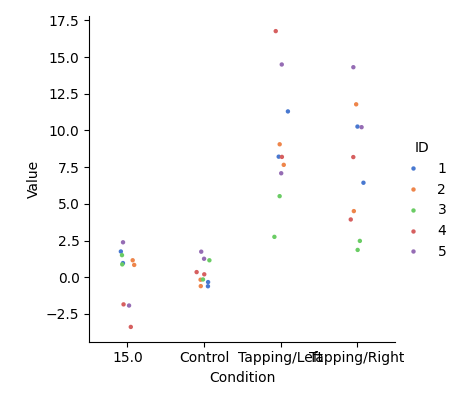
View individual results#
This figure simply summarises the information in the dataframe created above. We observe that the values extracted from the waveform for the control condition generally sit around 0. Whereas the tapping conditions have larger values. There is quite some variation in the values for the tapping conditions, which is typical of a group-level result. Many factors affect the response amplitude in an fNIRS experiment, including skin thickness and skull thickness, both of which vary across the head and across participants. For this reason, fNIRS is most appropriate for detecting changes within a single ROI between conditions.
<seaborn.axisgrid.FacetGrid object at 0x7fdb49a440d0>
Research question 1: Comparison of conditions#
In this example question we ask: is the HbO response in the left ROI to tapping with the right hand larger than the response when not tapping (control)? For this token example we subset the dataframe and then apply the mixed effect model.
input_data = df.query("Condition in ['Control', 'Tapping/Right']")
input_data = input_data.query("Chroma in ['hbo']")
input_data = input_data.query("ROI in ['Left_Hemisphere']")

roi_model = smf.mixedlm("Value ~ Condition", input_data, groups=input_data["ID"]).fit()
roi_model.summary()
The model indicates that for the oxyhaemoglobin (HbO) data in the left ROI, that the tapping condition with the right hand evokes a 9.0 μMol larger response than the control condition.
Research question 2: Are responses larger on the contralateral side to tapping?#
In this example question we ask: when tapping, is the brain region on the contralateral side of the brain to the tapping hand larger than the ipsilateral side?
First, the ROI data in the dataframe is encoded as ipsi- and contralateral to the tapping hand. Then the data is subset to just examine the two tapping conditions and the model is applied.
# Encode the ROIs as ipsi- or contralateral to the hand that is tapping.
df["Hemisphere"] = "Unknown"
df.loc[
    (df["Condition"] == "Tapping/Right") & (df["ROI"] == "Right_Hemisphere"),
    "Hemisphere",
] = "Ipsilateral"
df.loc[
    (df["Condition"] == "Tapping/Right") & (df["ROI"] == "Left_Hemisphere"),
    "Hemisphere",
] = "Contralateral"
df.loc[
    (df["Condition"] == "Tapping/Left") & (df["ROI"] == "Left_Hemisphere"), "Hemisphere"
] = "Ipsilateral"
df.loc[
    (df["Condition"] == "Tapping/Left") & (df["ROI"] == "Right_Hemisphere"),
    "Hemisphere",
] = "Contralateral"

# Subset the data for example model
input_data = df.query("Condition in ['Tapping/Right', 'Tapping/Left']")
input_data = input_data.query("Chroma in ['hbo']")
assert len(input_data)

roi_model = smf.mixedlm("Value ~ Hemisphere", input_data, groups=input_data["ID"]).fit()
roi_model.summary()
The model indicates that for the oxyhaemoglobin (HbO) data, the ipsilateral responses are 4.2 μMol smaller than those on the contralateral side to the hand that is tapping.
Total running time of the script: (0 minutes 8.558 seconds)
Estimated memory usage: 431 MB