Extracting a weak narrowband source with DSS

Can bandpass-biased DSS recover a weak known 10-Hz spatial source from multichannel data containing broadband noise and stronger off-target oscillatory activity?

The target and distractor sensor-space contributions are known in this controlled example. The narrowband bias emphasizes variance in the target band, but a strong narrowband component is not automatically neural; the source identity is known here only because the substrate was constructed explicitly [1][2].

References

[1]

Jaakko Sarela and Harri Valpola. Denoising source separation. Journal of Machine Learning Research, 6(9):233–272, 2005. URL: https://jmlr.org/papers/v6/sarela05a.html.

[2]

Alain de Cheveigné and Jonathan Z. Simon. Denoising based on spatial filtering. Journal of Neuroscience Methods, 171(2):331–339, 2008. doi:10.1016/j.jneumeth.2008.03.015.

Construct a controlled narrowband mixture

import numpy as np

from mne_denoise.dss import narrowband_dss
from mne_denoise.qa import rms_change
from mne_denoise.viz import plot_psd_comparison, plot_signal_overlay

rng = np.random.default_rng(20260902)
sfreq = 200.0
duration = 12.0
n_channels = 8
n_times = int(round(sfreq * duration))
times = np.arange(n_times) / sfreq
target_frequency = 10.0
distractor_frequency = 22.0

target_topography = rng.standard_normal(n_channels)
target_topography /= np.linalg.norm(target_topography)
distractor_topography = rng.standard_normal(n_channels)
distractor_topography -= target_topography * np.dot(
    target_topography,
    distractor_topography,
)
distractor_topography /= np.linalg.norm(distractor_topography)

target_waveform = 0.45 * np.sin(2.0 * np.pi * target_frequency * times + 0.2)
distractor_waveform = 1.8 * np.sin(2.0 * np.pi * distractor_frequency * times - 0.5)
target_sensor = target_topography[:, np.newaxis] * target_waveform
distractor_sensor = distractor_topography[:, np.newaxis] * distractor_waveform
background = 0.65 * rng.standard_normal((n_channels, n_times))
observed = target_sensor + distractor_sensor + background

Fit the public high-level narrowband DSS route

n_components = 1
n_select = 1
model = narrowband_dss(
    sfreq=sfreq,
    freq=target_frequency,
    bandwidth=2.0,
    n_components=n_components,
    n_select=n_select,
    component_action="retain",
    normalize_input=False,
    center=False,
    verbose=False,
)
cleaned = model.fit_transform(observed)

Compare target recovery with target-band selectivity

target_projection_before = target_topography @ observed
target_projection_after = target_topography @ cleaned
distractor_projection_before = distractor_topography @ observed
distractor_projection_after = distractor_topography @ cleaned

target_scale = np.sqrt(np.mean(target_sensor**2))
noisy_target_error = rms_change(observed, target_sensor) / target_scale
cleaned_target_error = rms_change(cleaned, target_sensor) / target_scale
target_correlation_before = float(
    np.corrcoef(target_projection_before.ravel(), target_waveform.ravel())[0, 1]
)
target_correlation_after = float(
    np.corrcoef(target_projection_after.ravel(), target_waveform.ravel())[0, 1]
)
target_gain_before = np.dot(target_projection_before, target_waveform) / np.dot(
    target_waveform,
    target_waveform,
)
target_gain_after = np.dot(target_projection_after, target_waveform) / np.dot(
    target_waveform,
    target_waveform,
)
target_power_ratio_before = np.mean(target_projection_before**2) / np.mean(
    distractor_projection_before**2
)
target_power_ratio_after = np.mean(target_projection_after**2) / np.mean(
    distractor_projection_after**2
)
distractor_residual_ratio = np.sqrt(np.mean(distractor_projection_after**2)) / np.sqrt(
    np.mean(distractor_projection_before**2)
)

print("Controlled narrowband DSS")
print(f"Sampling frequency: {sfreq:.1f} Hz")
print(f"Duration: {duration:.1f} s")
print(f"Channel count: {n_channels}")
print(f"n_components: {n_components}")
print(f"n_select: {n_select}")
print(f"Target frequency: {target_frequency:.1f} Hz")
print(f"Distractor frequency: {distractor_frequency:.1f} Hz")
print(f"Noisy-to-target relative RMS error: {noisy_target_error:.4f}")
print(f"Cleaned-to-target relative RMS error: {cleaned_target_error:.4f}")
print(f"Target waveform correlation before: {target_correlation_before:.4f}")
print(f"Target waveform correlation after:  {target_correlation_after:.4f}")
print(f"Target template gain before: {target_gain_before:.4f}")
print(f"Target template gain after:  {target_gain_after:.4f}")
print(
    f"Target/distractor projected power ratio before: {target_power_ratio_before:.4f}"
)
print(f"Target/distractor projected power ratio after:  {target_power_ratio_after:.4f}")
print(f"Distractor projected residual ratio: {distractor_residual_ratio:.4f}")

Controlled narrowband DSS
Sampling frequency: 200.0 Hz
Duration: 12.0 s
Channel count: 8
n_components: 1
n_select: 1
Target frequency: 10.0 Hz
Distractor frequency: 22.0 Hz
Noisy-to-target relative RMS error: 6.9681
Cleaned-to-target relative RMS error: 2.0340
Target waveform correlation before: 0.4375
Target waveform correlation after:  0.4387
Target template gain before: 0.9874
Target template gain after:  0.9854
Target/distractor projected power ratio before: 0.2608
Target/distractor projected power ratio after:  200.3465
Distractor projected residual ratio: 0.0359

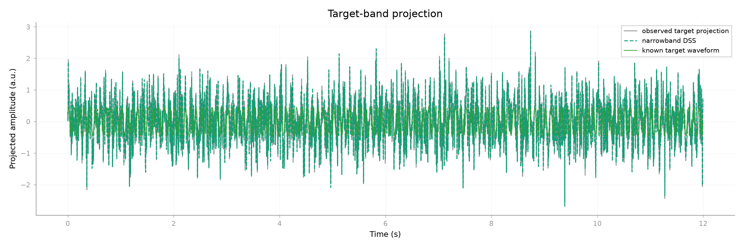
Inspect the target-recovery waveform

The target projection uses the predefined target topography, not a post-hoc channel choice. Amplitude is therefore shown without rescaling the after trace.

plot_signal_overlay(
    target_projection_before,
    target_projection_after,
    times,
    scale_after=False,
    before_label="observed target projection",
    after_label="narrowband DSS",
    reference=target_waveform,
    reference_label="known target waveform",
    x_label="Time (s)",
    y_label="Projected amplitude (a.u.)",
    title="Target-band projection",
    show=False,
)

<Figure size 2400x800 with 1 Axes>

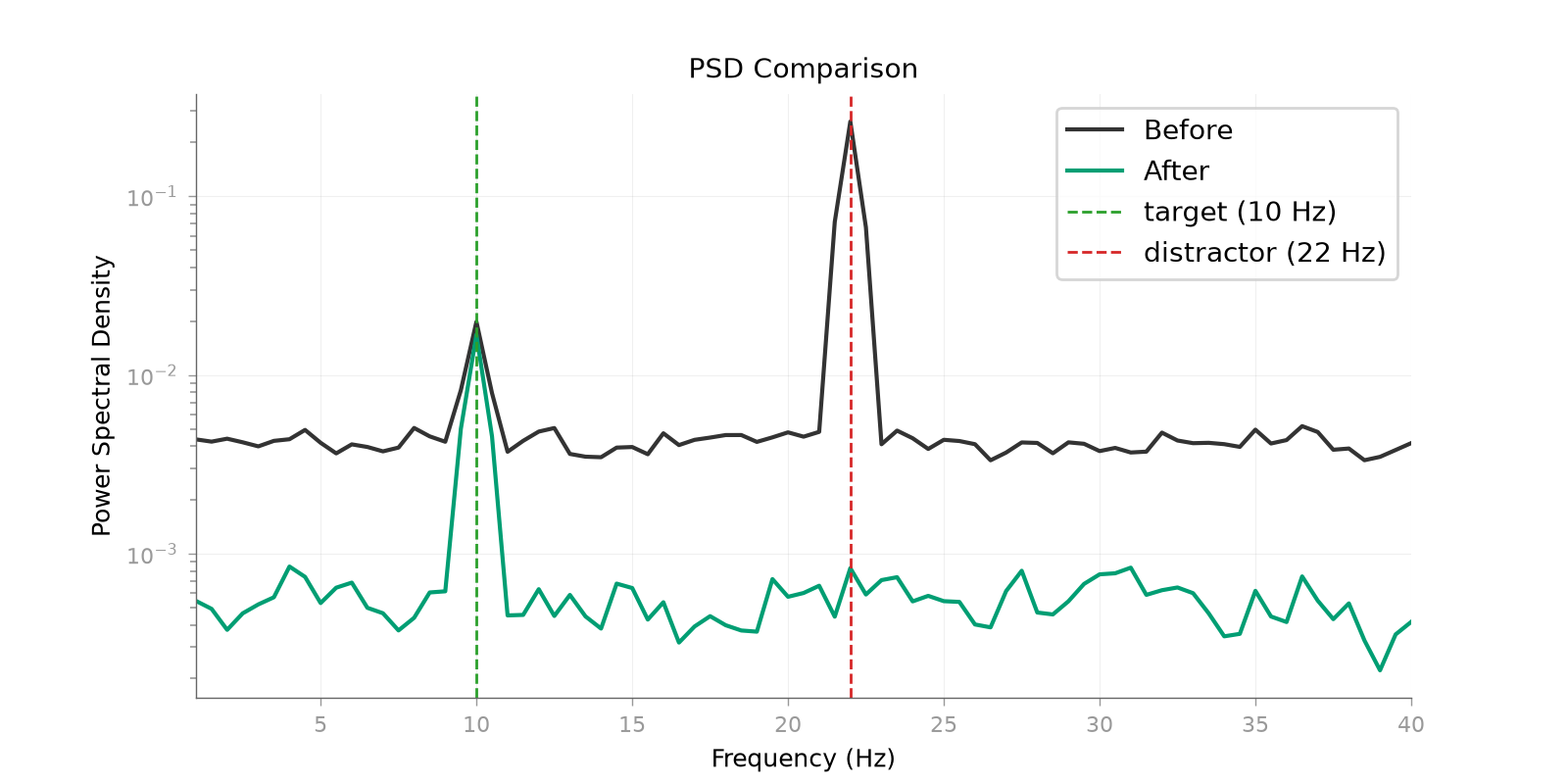
Compare the target and distractor spectra

psd_figure = plot_psd_comparison(
    observed,
    cleaned,
    sfreq=sfreq,
    fmin=1.0,
    fmax=40.0,
    show=False,
)
psd_axis = psd_figure.axes[0]
psd_axis.axvline(
    target_frequency,
    color="tab:green",
    linestyle="--",
    linewidth=1.0,
    label="target (10 Hz)",
)
psd_axis.axvline(
    distractor_frequency,
    color="tab:red",
    linestyle="--",
    linewidth=1.0,
    label="distractor (22 Hz)",
)
psd_axis.legend(loc="upper right")

<matplotlib.legend.Legend object at 0x7f265fdb2210>

Interpretation

The retained component is ranked by variance emphasized by the 10-Hz bandpass bias. The target projection and the target/distractor ratio test whether that bias selected the known source rather than merely reducing broadband variance. In recorded data, a strong narrowband component still needs an independent scientific interpretation.