
Examples#
The examples below show how mne-denoise methods can be used for specific
scientific denoising problems in EEG and MEG.
Each example starts from the structure that makes a method appropriate: clean calibration data, spatial redundancy, a forward model, spectral structure, repeated trials, or reference channels. Where possible, examples evaluate both suppression of the target artifact and preservation of the signal of interest.
Controlled simulations and deliberately contaminated recordings are used when ground truth is needed. Real MNE datasets are used when sensor geometry, recording structure, or container behavior is scientifically relevant.
The examples are demonstrations, not universal benchmarks or parameter recommendations. Parameters should be validated for the recording and scientific endpoint at hand.
ASR#
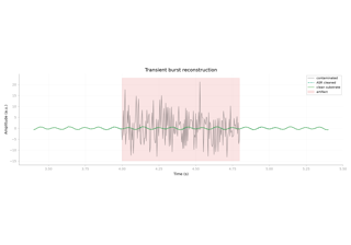
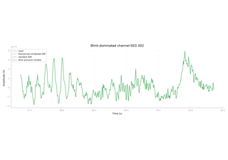
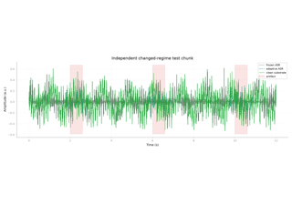
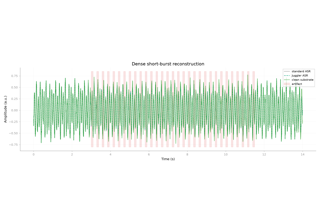
These examples cover four distinct ASR use cases: transient burst repair with standard ASR, Riemannian calibration for blink-contaminated EEG, adaptive calibration when recording statistics change, and Juggler-style reference selection when clean windows are scarce.
The examples use controlled data when signal preservation requires ground truth and real EEG when the recording context itself is informative. Comparisons are illustrative rather than universal benchmarks.
SNS#
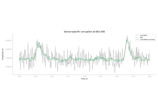
This example uses a real EEG recording with deliberately added sensor-specific noise to show the assumption behind Sensor Noise Suppression: signals represented redundantly across sensors can be used to reconstruct noise that is specific to individual channels.
Because the unmodified recording is available as a reference substrate, the example evaluates both recovery of the corrupted channels and change on untouched channels.
SOUND#
This example uses the MNE Sample EEG recording and its public forward solution to show how forward-model information can estimate channel-specific noise. Known planted corruption provides an artifact-recovery endpoint, while applying the same fitted operator to the unmodified recording provides a signal-preservation control.
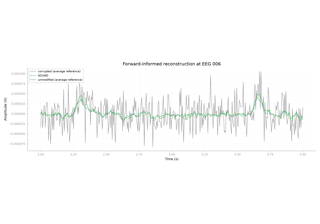
Forward-informed sensor-noise suppression with SOUND
Spectrum interpolation#
This example uses controlled nonstationary 60-Hz interference with abrupt changes in amplitude to illustrate the use case for spectrum interpolation.
Known clean data provide a time-domain preservation reference, and a public notch filter is included only as a contextual comparison. The example evaluates line attenuation and signal distortion separately.
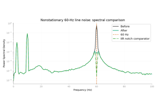
Removing nonstationary line noise with spectrum interpolation
ZapLine#
These examples illustrate two distinct line-noise settings.
The first applies standard ZapLine to real MNE Sample MEG with a stable 60-Hz target and evaluates line attenuation together with off-band spectral change.
The second uses controlled nonstationary frequency-specific noise to compare a single global fit with adaptive ZapLine. Known clean data make it possible to evaluate reconstruction and signal preservation separately.
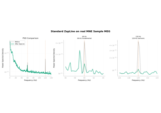
Removing 60-Hz line noise and its harmonic from real MEG with ZapLine
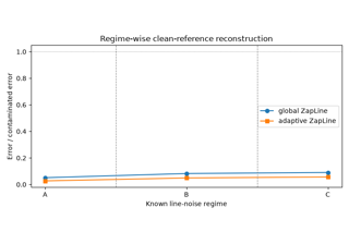
Adaptive ZapLine for changing line-noise statistics
DSS#
These examples show four scientifically distinct ways to define structure of interest with Denoising Source Separation.
The evoked example uses trial reproducibility on real held-out somatosensory MEG data. The cardiac example combines real Sample EEG and real R-peak timing with a controlled planted cardiac artifact, then uses an independent clean-input preservation control. The narrowband example uses controlled spectral structure to recover a known target source. The TimeShiftDSS example extends reproducibility into lag-augmented spatiotemporal space and uses held-out and surrogate validation.
A DSS bias defines what the decomposition emphasizes; it does not by itself establish that a selected component is neural signal or artifact.
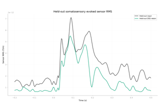
Enhancing a reproducible somatosensory response with DSS
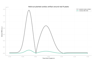
Removing a planted cardiac-locked artifact with DSS
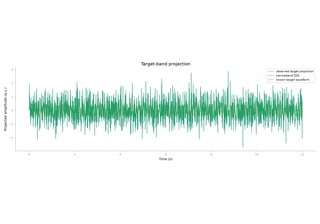
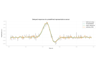
Recovering delayed reproducible structure with TimeShiftDSS
SSA#
The first example shows additive Basic SSA decomposition and an mne-denoise-specific frequency-guided grouping rule on a controlled slow-drift problem.
The second illustrates local SSA for a high-amplitude single-channel EOG-like artifact. Known clean structure is retained so artifact recovery and neural transient preservation can be evaluated separately.
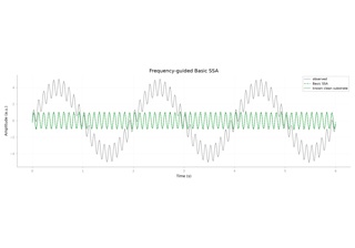
Basic SSA decomposition with frequency-guided grouping
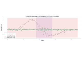
Removing a high-amplitude single-channel artifact with local SSA
BSS-CCA#
This example uses a real EEG substrate with controlled broadband muscle-like contamination to illustrate reference-free BSS-CCA. The method separates components according to lagged temporal correlation, so broadband low-correlation components can be attenuated without a dedicated reference channel.
The controlled construction makes it possible to evaluate both artifact recovery and change outside the contaminated periods. Low lagged correlation is a selection heuristic, not an automatic artifact label.
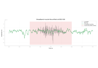
Attenuating broadband muscle artifact with BSS-CCA
iCanClean#
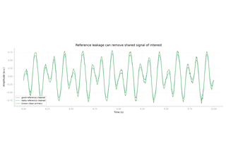
This example demonstrates reference-informed CCA cleaning with iCanClean using a controlled recording in which the artifact and signal of interest are known.
Two reference conditions are compared: one that primarily captures the artifact and one that also contains signal of interest. The comparison illustrates why shared variance is not, by itself, evidence that a component should be removed.
SSP-SIR#
This example uses a real MNE Sample EEG evoked response as a clean methodological substrate and adds a controlled short TMS-like muscle artifact.
The artifact direction is constructed with known spatial overlap with a clean response topography. SSP-SIR is then evaluated with separate artifact attenuation and clean-input preservation controls using a public MNE forward solution.
The example is a controlled illustration, not validation on real TMS-EEG.
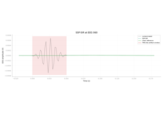
Suppressing a TMS-like muscle artifact with SSP-SIR