Adaptive ZapLine for changing line-noise statistics

When line-noise frequency, strength, or spatial pattern changes over time, does adaptive ZapLine provide a better controlled reconstruction than one global ZapLine fit? Three known regimes make it possible to compare artifact recovery with a separate 10-Hz target-signal preservation endpoint.

ZapLine combines spectral and spatial filtering [1], while Zapline-plus motivates chunk-wise adaptation to changing frequency-specific noise statistics [2]. Adaptive processing is therefore an additional assumption about nonstationarity, not a universal replacement for a global fit.

References

[1]

Alain de Cheveigné. Zapline: a simple and effective method to remove power line artifacts. NeuroImage, 207:116356, 2020. doi:10.1016/j.neuroimage.2019.116356.

[2]

Marius Klug and Niels A. Kloosterman. Zapline-plus: a zapline extension for automatic and adaptive removal of frequency-specific noise artifacts in m/eeg. Human Brain Mapping, 43(9):2743–2758, 2022. doi:10.1002/hbm.25832.

Construct a controlled three-regime recording

import matplotlib.pyplot as plt
import numpy as np

from mne_denoise.qa import rms_change
from mne_denoise.viz import plot_psd_comparison
from mne_denoise.zapline import ZapLine

sfreq = 200.0
duration = 90.0
n_channels = 8
n_times = int(round(duration * sfreq))
times = np.arange(n_times) / sfreq
rng = np.random.default_rng(20260902)

# The clean substrate is one continuous background-plus-target process shared by
# all regimes. The 10-Hz component is a known signal-of-interest template.
channel_phases = rng.uniform(0.0, 2.0 * np.pi, n_channels)
background = 0.08 * rng.standard_normal((n_channels, n_times)) + 0.12 * np.sin(
    2.0 * np.pi * 3.0 * times[None, :] + channel_phases[:, None]
)
target_pattern = rng.standard_normal(n_channels)
target_pattern /= np.linalg.norm(target_pattern)
target_wave = 0.35 * np.sin(2.0 * np.pi * 10.0 * times)
target_template = target_pattern[:, None] * target_wave[None, :]
clean_reference = background + target_template

# Use distinct, fixed spatial patterns to make the nonstationarity explicit.
topography_a = np.array([1.0, 0.8, 0.6, 0.4, 0.2, 0.1, 0.05, 0.02])
topography_b = topography_a[::-1].copy()
topography_c = np.array([1.0, -1.0, 1.0, -1.0, 1.0, -1.0, 1.0, -1.0])
topographies = (topography_a, topography_b, topography_c)
for topography in topographies:
    topography /= np.linalg.norm(topography)

regimes = (
    ("A", 0.0, 30.0, 50.00, 4.0, topography_a),
    ("B", 30.0, 60.0, 50.05, 2.5, topography_b),
    ("C", 60.0, 90.0, 49.95, 3.0, topography_c),
)
line_artifact = np.zeros_like(clean_reference)
for name, start, stop, frequency, amplitude, topography in regimes:
    interval = slice(int(start * sfreq), int(stop * sfreq))
    envelope = np.ones(interval.stop - interval.start)
    if name == "C":
        # The final regime has a weaker baseline with stronger bursts and is
        # spatially distinct.
        local_times = times[interval]
        envelope = 0.25 + 0.75 * (
            ((local_times >= 64.0) & (local_times < 72.0))
            | ((local_times >= 78.0) & (local_times < 86.0))
        )
    source = amplitude * envelope * np.sin(2.0 * np.pi * frequency * times[interval])
    line_artifact[:, interval] = topography[:, None] * source[None, :]

contaminated = clean_reference + line_artifact

Compare one global fit with the adaptive public estimator

global_model = ZapLine(
    sfreq=sfreq,
    line_freq=50.0,
    n_select="auto",
    verbose=False,
)
global_clean = global_model.fit_transform(contaminated)

adaptive_model = ZapLine(
    sfreq=sfreq,
    line_freq=50.0,
    adaptive=True,
    verbose=False,
)
adaptive_clean = adaptive_model.fit_transform(contaminated)

Evaluate recovery by regime and preserve an independent target endpoint

regime_labels = []
global_ratios = []
adaptive_ratios = []
print("Known-regime reconstruction errors:")
for name, start, stop, frequency, _amplitude, _topography in regimes:
    interval = slice(int(start * sfreq), int(stop * sfreq))
    contaminated_error = rms_change(
        contaminated[:, interval], clean_reference[:, interval]
    )
    global_error = rms_change(global_clean[:, interval], clean_reference[:, interval])
    adaptive_error = rms_change(
        adaptive_clean[:, interval], clean_reference[:, interval]
    )
    global_ratio = global_error / contaminated_error
    adaptive_ratio = adaptive_error / contaminated_error
    regime_labels.append(name)
    global_ratios.append(global_ratio)
    adaptive_ratios.append(adaptive_ratio)
    regime_target_template = target_template[:, interval]
    regime_target_energy = np.sum(regime_target_template**2)
    regime_reference_projection = (
        np.sum(clean_reference[:, interval] * regime_target_template)
        / regime_target_energy
    )
    regime_global_projection = (
        np.sum(global_clean[:, interval] * regime_target_template)
        / regime_target_energy
    )
    regime_adaptive_projection = (
        np.sum(adaptive_clean[:, interval] * regime_target_template)
        / regime_target_energy
    )
    regime_global_gain = regime_global_projection / regime_reference_projection
    regime_adaptive_gain = regime_adaptive_projection / regime_reference_projection
    print(
        f"  Regime {name} ({start:.0f}-{stop:.0f} s, {frequency:.2f} Hz): "
        f"contaminated error={contaminated_error:.4f}; "
        f"global error={global_error:.4f}, residual ratio={global_ratio:.3f}; "
        f"adaptive error={adaptive_error:.4f}, residual ratio={adaptive_ratio:.3f}"
    )
    print(
        f"  Regime {name} target gain — global / adaptive: "
        f"{regime_global_gain:.3f} / {regime_adaptive_gain:.3f}"
    )

# Project the known 10-Hz component, rather than treating lower 50-Hz power as
# evidence of preservation. Adaptive mode is transductive, so this uses the
# clean-reference reconstruction endpoint instead of a second transform call.
target_energy = np.sum(target_template**2)
reference_target_projection = np.sum(clean_reference * target_template) / target_energy
global_target_projection = np.sum(global_clean * target_template) / target_energy
adaptive_target_projection = np.sum(adaptive_clean * target_template) / target_energy
global_target_gain = global_target_projection / reference_target_projection
adaptive_target_gain = adaptive_target_projection / reference_target_projection

chunk_info = adaptive_model.adaptive_results_["chunk_info"]
reported_frequencies = sorted(
    {
        round(float(chunk["fine_freq"]), 2)
        for chunk in chunk_info
        if chunk.get("fine_freq") is not None
    }
)
print(f"Global components removed: {global_model.n_removed_}")
print(
    f"Adaptive segment/component passes: {len(chunk_info)} segments / "
    f"{adaptive_model.n_removed_} component passes"
)
print(f"Adaptive reported segment frequencies (Hz): {reported_frequencies}")
print(f"10-Hz target-signal retention - global:   {global_target_gain:.3f}")
print(f"10-Hz target-signal retention - adaptive: {adaptive_target_gain:.3f}")

Known-regime reconstruction errors:
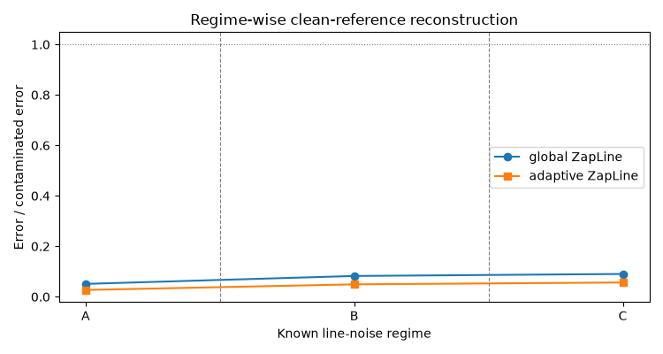
  Regime A (0-30 s, 50.00 Hz): contaminated error=1.0000; global error=0.0510, residual ratio=0.051; adaptive error=0.0270, residual ratio=0.027
  Regime A target gain — global / adaptive: 0.934 / 0.998
  Regime B (30-60 s, 50.05 Hz): contaminated error=0.6250; global error=0.0515, residual ratio=0.082; adaptive error=0.0307, residual ratio=0.049
  Regime B target gain — global / adaptive: 0.936 / 0.978
  Regime C (60-90 s, 49.95 Hz): contaminated error=0.5625; global error=0.0508, residual ratio=0.090; adaptive error=0.0318, residual ratio=0.057
  Regime C target gain — global / adaptive: 0.931 / 0.989
Global components removed: 3
Adaptive segment/component passes: 3 segments / 3 component passes
Adaptive reported segment frequencies (Hz): [49.95, 50.0, 50.04]
10-Hz target-signal retention - global:   0.934
10-Hz target-signal retention - adaptive: 0.989

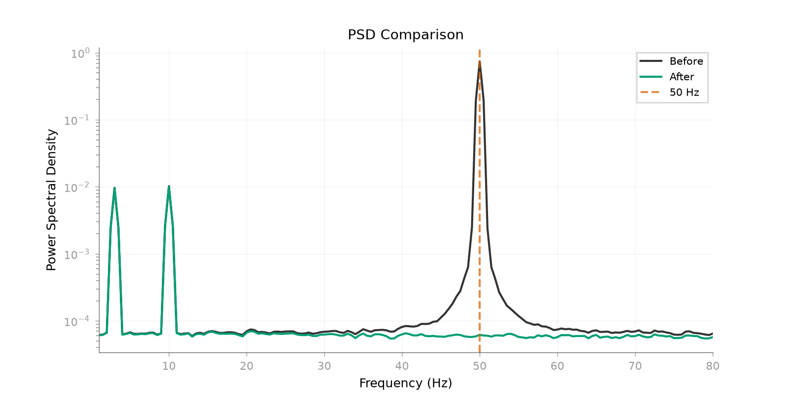
Inspect the adaptive spectrum

plot_psd_comparison(
    contaminated,
    adaptive_clean,
    sfreq=sfreq,
    fmin=1.0,
    fmax=80.0,
    line_freq=50.0,
    show=False,
)

<Figure size 1600x800 with 1 Axes>

Compare regime-wise reconstruction

The public PSD helper cannot express a known-clean, regime-wise residual ratio, so this small custom plot shows that endpoint and the boundaries.

fig, ax = plt.subplots(figsize=(7.5, 4.0))
centers = np.array([15.0, 45.0, 75.0])
ax.plot(centers, global_ratios, "o-", label="global ZapLine")
ax.plot(centers, adaptive_ratios, "s-", label="adaptive ZapLine")
for boundary in (30.0, 60.0):
    ax.axvline(boundary, color="0.5", linestyle="--", linewidth=0.8)
ax.axhline(1.0, color="0.5", linestyle=":", linewidth=0.8)
ax.set_xticks(centers)
ax.set_xticklabels(regime_labels)
ax.set_xlabel("Known line-noise regime")
ax.set_ylabel("Error / contaminated error")
ax.set_title("Regime-wise clean-reference reconstruction")
ax.legend()
fig.tight_layout()