Explore event-related dynamics for specific frequency bands

The objective is to show you how to explore spectrally localized effects. For this purpose we adapt the method described in 1 and use it on the somato dataset. The idea is to track the band-limited temporal evolution of spatial patterns by using the global field power (GFP).

We first bandpass filter the signals and then apply a Hilbert transform. To reveal oscillatory activity the evoked response is then subtracted from every single trial. Finally, we rectify the signals prior to averaging across trials by taking the magniude of the Hilbert. Then the GFP is computed as described in 2, using the sum of the squares but without normalization by the rank. Baselining is subsequently applied to make the GFP comparable between frequencies. The procedure is then repeated for each frequency band of interest and all GFPs are visualized. To estimate uncertainty, non-parametric confidence intervals are computed as described in 3 across channels.

The advantage of this method over summarizing the Space x Time x Frequency output of a Morlet Wavelet in frequency bands is relative speed and, more importantly, the clear-cut comparability of the spectral decomposition (the same type of filter is used across all bands).

We will use this dataset: Somatosensory

References

1

Riitta Hari and Riitta Salmelin. Human cortical oscillations: a neuromagnetic view through the skull. Trends in Neurosciences, 20(1):44–49, 1997. doi:10.1016/S0166-2236(96)10065-5.

2

Denis A. Engemann and Alexandre Gramfort. Automated model selection in covariance estimation and spatial whitening of MEG and EEG signals. NeuroImage, 108:328–342, 2015. doi:10.1016/j.neuroimage.2014.12.040.

3

Bradley Efron and Trevor Hastie. Computer Age Statistical Inference: Algorithms, Evidence, and Data Science. Number 5 in Institute of Mathematical Statistics Monographs. Cambridge University Press, New York, 2016. ISBN 978-1-107-14989-2. URL: https://web.stanford.edu/~hastie/CASI/.

# Authors: Denis A. Engemann <denis.engemann@gmail.com>
#          Stefan Appelhoff <stefan.appelhoff@mailbox.org>
#
# License: BSD (3-clause)
import os.path as op

import numpy as np
import matplotlib.pyplot as plt

import mne
from mne.datasets import somato
from mne.baseline import rescale
from mne.stats import bootstrap_confidence_interval

Set parameters

data_path = somato.data_path()
subject = '01'
task = 'somato'
raw_fname = op.join(data_path, 'sub-{}'.format(subject), 'meg',
                    'sub-{}_task-{}_meg.fif'.format(subject, task))

# let's explore some frequency bands
iter_freqs = [
    ('Theta', 4, 7),
    ('Alpha', 8, 12),
    ('Beta', 13, 25),
    ('Gamma', 30, 45)
]

We create average power time courses for each frequency band

# set epoching parameters
event_id, tmin, tmax = 1, -1., 3.
baseline = None

# get the header to extract events
raw = mne.io.read_raw_fif(raw_fname)
events = mne.find_events(raw, stim_channel='STI 014')

frequency_map = list()

for band, fmin, fmax in iter_freqs:
    # (re)load the data to save memory
    raw = mne.io.read_raw_fif(raw_fname)
    raw.pick_types(meg='grad', eog=True)  # we just look at gradiometers
    raw.load_data()

    # bandpass filter
    raw.filter(fmin, fmax, n_jobs=1,  # use more jobs to speed up.
               l_trans_bandwidth=1,  # make sure filter params are the same
               h_trans_bandwidth=1)  # in each band and skip "auto" option.

    # epoch
    epochs = mne.Epochs(raw, events, event_id, tmin, tmax, baseline=baseline,
                        reject=dict(grad=4000e-13, eog=350e-6),
                        preload=True)
    # remove evoked response
    epochs.subtract_evoked()

    # get analytic signal (envelope)
    epochs.apply_hilbert(envelope=True)
    frequency_map.append(((band, fmin, fmax), epochs.average()))
    del epochs
del raw

Out:

Opening raw data file /home/circleci/mne_data/MNE-somato-data/sub-01/meg/sub-01_task-somato_meg.fif...
    Range : 237600 ... 506999 =    791.189 ...  1688.266 secs
Ready.
111 events found
Event IDs: [1]
Opening raw data file /home/circleci/mne_data/MNE-somato-data/sub-01/meg/sub-01_task-somato_meg.fif...
    Range : 237600 ... 506999 =    791.189 ...  1688.266 secs
Ready.
Reading 0 ... 269399  =      0.000 ...   897.077 secs...
Filtering raw data in 1 contiguous segment
Setting up band-pass filter from 4 - 7 Hz

FIR filter parameters
---------------------
Designing a one-pass, zero-phase, non-causal bandpass filter:
- Windowed time-domain design (firwin) method
- Hamming window with 0.0194 passband ripple and 53 dB stopband attenuation
- Lower passband edge: 4.00
- Lower transition bandwidth: 1.00 Hz (-6 dB cutoff frequency: 3.50 Hz)
- Upper passband edge: 7.00 Hz
- Upper transition bandwidth: 1.00 Hz (-6 dB cutoff frequency: 7.50 Hz)
- Filter length: 993 samples (3.307 sec)

Not setting metadata
Not setting metadata
111 matching events found
No baseline correction applied
0 projection items activated
Loading data for 111 events and 1202 original time points ...
    Rejecting  epoch based on EOG : ['EOG 061']
    Rejecting  epoch based on EOG : ['EOG 061']
    Rejecting  epoch based on EOG : ['EOG 061']
3 bad epochs dropped
Subtracting Evoked from Epochs
    The following channels are not included in the subtraction: EOG 061
[done]
Opening raw data file /home/circleci/mne_data/MNE-somato-data/sub-01/meg/sub-01_task-somato_meg.fif...
    Range : 237600 ... 506999 =    791.189 ...  1688.266 secs
Ready.
Reading 0 ... 269399  =      0.000 ...   897.077 secs...
Filtering raw data in 1 contiguous segment
Setting up band-pass filter from 8 - 12 Hz

FIR filter parameters
---------------------
Designing a one-pass, zero-phase, non-causal bandpass filter:
- Windowed time-domain design (firwin) method
- Hamming window with 0.0194 passband ripple and 53 dB stopband attenuation
- Lower passband edge: 8.00
- Lower transition bandwidth: 1.00 Hz (-6 dB cutoff frequency: 7.50 Hz)
- Upper passband edge: 12.00 Hz
- Upper transition bandwidth: 1.00 Hz (-6 dB cutoff frequency: 12.50 Hz)
- Filter length: 993 samples (3.307 sec)

Not setting metadata
Not setting metadata
111 matching events found
No baseline correction applied
0 projection items activated
Loading data for 111 events and 1202 original time points ...
    Rejecting  epoch based on EOG : ['EOG 061']
    Rejecting  epoch based on EOG : ['EOG 061']
    Rejecting  epoch based on EOG : ['EOG 061']
3 bad epochs dropped
Subtracting Evoked from Epochs
    The following channels are not included in the subtraction: EOG 061
[done]
Opening raw data file /home/circleci/mne_data/MNE-somato-data/sub-01/meg/sub-01_task-somato_meg.fif...
    Range : 237600 ... 506999 =    791.189 ...  1688.266 secs
Ready.
Reading 0 ... 269399  =      0.000 ...   897.077 secs...
Filtering raw data in 1 contiguous segment
Setting up band-pass filter from 13 - 25 Hz

FIR filter parameters
---------------------
Designing a one-pass, zero-phase, non-causal bandpass filter:
- Windowed time-domain design (firwin) method
- Hamming window with 0.0194 passband ripple and 53 dB stopband attenuation
- Lower passband edge: 13.00
- Lower transition bandwidth: 1.00 Hz (-6 dB cutoff frequency: 12.50 Hz)
- Upper passband edge: 25.00 Hz
- Upper transition bandwidth: 1.00 Hz (-6 dB cutoff frequency: 25.50 Hz)
- Filter length: 993 samples (3.307 sec)

Not setting metadata
Not setting metadata
111 matching events found
No baseline correction applied
0 projection items activated
Loading data for 111 events and 1202 original time points ...
    Rejecting  epoch based on EOG : ['EOG 061']
    Rejecting  epoch based on EOG : ['EOG 061']
    Rejecting  epoch based on EOG : ['EOG 061']
3 bad epochs dropped
Subtracting Evoked from Epochs
    The following channels are not included in the subtraction: EOG 061
[done]
Opening raw data file /home/circleci/mne_data/MNE-somato-data/sub-01/meg/sub-01_task-somato_meg.fif...
    Range : 237600 ... 506999 =    791.189 ...  1688.266 secs
Ready.
Reading 0 ... 269399  =      0.000 ...   897.077 secs...
Filtering raw data in 1 contiguous segment
Setting up band-pass filter from 30 - 45 Hz

FIR filter parameters
---------------------
Designing a one-pass, zero-phase, non-causal bandpass filter:
- Windowed time-domain design (firwin) method
- Hamming window with 0.0194 passband ripple and 53 dB stopband attenuation
- Lower passband edge: 30.00
- Lower transition bandwidth: 1.00 Hz (-6 dB cutoff frequency: 29.50 Hz)
- Upper passband edge: 45.00 Hz
- Upper transition bandwidth: 1.00 Hz (-6 dB cutoff frequency: 45.50 Hz)
- Filter length: 993 samples (3.307 sec)

Not setting metadata
Not setting metadata
111 matching events found
No baseline correction applied
0 projection items activated
Loading data for 111 events and 1202 original time points ...
    Rejecting  epoch based on EOG : ['EOG 061']
    Rejecting  epoch based on EOG : ['EOG 061']
    Rejecting  epoch based on EOG : ['EOG 061']
3 bad epochs dropped
Subtracting Evoked from Epochs
    The following channels are not included in the subtraction: EOG 061
[done]

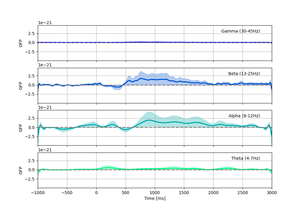
Now we can compute the Global Field Power We can track the emergence of spatial patterns compared to baseline for each frequency band, with a bootstrapped confidence interval.

We see dominant responses in the Alpha and Beta bands.

# Helper function for plotting spread
def stat_fun(x):
    """Return sum of squares."""
    return np.sum(x ** 2, axis=0)


# Plot
fig, axes = plt.subplots(4, 1, figsize=(10, 7), sharex=True, sharey=True)
colors = plt.get_cmap('winter_r')(np.linspace(0, 1, 4))
for ((freq_name, fmin, fmax), average), color, ax in zip(
        frequency_map, colors, axes.ravel()[::-1]):
    times = average.times * 1e3
    gfp = np.sum(average.data ** 2, axis=0)
    gfp = mne.baseline.rescale(gfp, times, baseline=(None, 0))
    ax.plot(times, gfp, label=freq_name, color=color, linewidth=2.5)
    ax.axhline(0, linestyle='--', color='grey', linewidth=2)
    ci_low, ci_up = bootstrap_confidence_interval(average.data, random_state=0,
                                                  stat_fun=stat_fun)
    ci_low = rescale(ci_low, average.times, baseline=(None, 0))
    ci_up = rescale(ci_up, average.times, baseline=(None, 0))
    ax.fill_between(times, gfp + ci_up, gfp - ci_low, color=color, alpha=0.3)
    ax.grid(True)
    ax.set_ylabel('GFP')
    ax.annotate('%s (%d-%dHz)' % (freq_name, fmin, fmax),
                xy=(0.95, 0.8),
                horizontalalignment='right',
                xycoords='axes fraction')
    ax.set_xlim(-1000, 3000)

axes.ravel()[-1].set_xlabel('Time [ms]')

Out:

Applying baseline correction (mode: mean)
Applying baseline correction (mode: mean)
Applying baseline correction (mode: mean)
Applying baseline correction (mode: mean)
Applying baseline correction (mode: mean)
Applying baseline correction (mode: mean)
Applying baseline correction (mode: mean)
Applying baseline correction (mode: mean)
Applying baseline correction (mode: mean)
Applying baseline correction (mode: mean)
Applying baseline correction (mode: mean)
Applying baseline correction (mode: mean)

Estimated memory usage: 830 MB

Compute and visualize ERDS maps Time-frequency on simulated data (Multitaper vs. Morlet vs. Stockwell)