Note
Click here to download the full example code
Working with ECoG data
MNE supports working with more than just MEG and EEG data. Here we show some of the functions that can be used to facilitate working with electrocorticography (ECoG) data.
This example shows how to use:
ECoG data (available here) from an epilepsy patient during a seizure
channel locations in FreeSurfer’s
fsaverageMRI spaceprojection onto a pial surface
For a complementary example that involves sEEG data, channel locations in MNI space, or projection into a volume, see Working with sEEG data.
# Authors: Eric Larson <larson.eric.d@gmail.com>
# Chris Holdgraf <choldgraf@gmail.com>
# Adam Li <adam2392@gmail.com>
# Alex Rockhill <aprockhill@mailbox.org>
# Liberty Hamilton <libertyhamilton@gmail.com>
#
# License: BSD (3-clause)
import os.path as op
import numpy as np
import matplotlib.pyplot as plt
from matplotlib.cm import get_cmap
from mne_bids import BIDSPath, read_raw_bids
import mne
from mne.viz import plot_alignment, snapshot_brain_montage
print(__doc__)
# paths to mne datasets - sample ECoG and FreeSurfer subject
bids_root = mne.datasets.epilepsy_ecog.data_path()
sample_path = mne.datasets.sample.data_path()
subjects_dir = op.join(sample_path, 'subjects')
Load in data and perform basic preprocessing
Let’s load some ECoG electrode data with mne-bids.
# first define the bids path
bids_path = BIDSPath(root=bids_root, subject='pt1', session='presurgery',
task='ictal', datatype='ieeg', extension='vhdr')
# then we'll use it to load in the sample dataset
# Here we use a format (iEEG) that is only available in MNE-BIDS 0.7+, so it
# will emit a warning on versions <= 0.6
raw = read_raw_bids(bids_path=bids_path, verbose=False)
# Pick only the ECoG channels, removing the EKG channels
raw.pick_types(ecog=True)
# Load the data
raw.load_data()
# Then we remove line frequency interference
raw.notch_filter([60], trans_bandwidth=3)
# drop bad channels
raw.drop_channels(raw.info['bads'])
# the coordinate frame of the montage
print(raw.get_montage().get_positions()['coord_frame'])
# Find the annotated events
events, event_id = mne.events_from_annotations(raw)
# Make a 25 second epoch that spans before and after the seizure onset
epoch_length = 25 # seconds
epochs = mne.Epochs(raw, events, event_id=event_id['onset'],
tmin=13, tmax=13 + epoch_length, baseline=None)
# And then load data and downsample.
# .. note: This is just to save execution time in this example, you should
# not need to do this in general!
epochs.load_data()
epochs.resample(200) # Hz, will also load the data for us
# Finally, make evoked from the one epoch
evoked = epochs.average()
Out:
Extracting parameters from /home/circleci/mne_data/MNE-epilepsy-ecog-data/sub-pt1/ses-presurgery/ieeg/sub-pt1_ses-presurgery_task-ictal_ieeg.vhdr...
Setting channel info structure...
Reading events from /home/circleci/mne_data/MNE-epilepsy-ecog-data/sub-pt1/ses-presurgery/ieeg/sub-pt1_ses-presurgery_task-ictal_events.tsv.
Reading channel info from /home/circleci/mne_data/MNE-epilepsy-ecog-data/sub-pt1/ses-presurgery/ieeg/sub-pt1_ses-presurgery_task-ictal_channels.tsv.
Reading electrode coords from /home/circleci/mne_data/MNE-epilepsy-ecog-data/sub-pt1/ses-presurgery/ieeg/sub-pt1_ses-presurgery_space-fsaverage_electrodes.tsv.
/home/circleci/.local/lib/python3.8/site-packages/mne_bids/dig.py:521: RuntimeWarning: Fiducial point nasion not found, assuming identity unknown to head transformation
raw.set_montage(montage, on_missing='warn', verbose=verbose)
/home/circleci/.local/lib/python3.8/site-packages/mne_bids/dig.py:521: RuntimeWarning: DigMontage is only a subset of info. There are 3 channel positions not present in the DigMontage. The required channels are:
['RQ1', 'RQ2', 'N/A'].
Consider using inst.set_channel_types if these are not EEG channels, or use the on_missing parameter if the channel positions are allowed to be unknown in your analyses.
raw.set_montage(montage, on_missing='warn', verbose=verbose)
Reading 0 ... 269079 = 0.000 ... 269.079 secs...
Setting up band-stop filter from 58 - 62 Hz
FIR filter parameters
---------------------
Designing a one-pass, zero-phase, non-causal bandstop filter:
- Windowed time-domain design (firwin) method
- Hamming window with 0.0194 passband ripple and 53 dB stopband attenuation
- Lower passband edge: 58.35
- Lower transition bandwidth: 1.50 Hz (-6 dB cutoff frequency: 57.60 Hz)
- Upper passband edge: 61.65 Hz
- Upper transition bandwidth: 1.50 Hz (-6 dB cutoff frequency: 62.40 Hz)
- Filter length: 2201 samples (2.201 sec)
mni_tal
Used Annotations descriptions: ['AD1-4, ATT1,2', 'AST1,3', 'G16', 'PD', 'SLT1-3', 'offset', 'onset']
Not setting metadata
Not setting metadata
1 matching events found
No baseline correction applied
0 projection items activated
Loading data for 1 events and 25001 original time points ...
0 bad epochs dropped
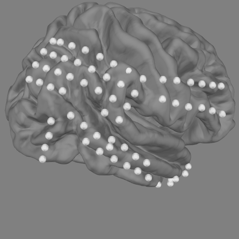
Explore the electrodes on a template brain
Our electrodes are shown after being morphed to fsaverage brain so we’ll use
this fsaverage brain to plot the locations of our electrodes. We’ll use
snapshot_brain_montage() to save the plot as image data
(along with xy positions of each electrode in the image), so that later
we can plot frequency band power on top of it.
fig = plot_alignment(raw.info, subject='fsaverage', subjects_dir=subjects_dir,
surfaces=['pial'], coord_frame='mri')
az, el, focalpoint = 160, -70, [0.067, -0.040, 0.018]
mne.viz.set_3d_view(fig, azimuth=az, elevation=el, focalpoint=focalpoint)
xy, im = snapshot_brain_montage(fig, raw.info)

Out:
Plotting 84 ECoG locations
Compute frequency features of the data
Next, we’ll compute the signal power in the gamma (30-90 Hz) band, downsampling the result to 10 Hz (to save time).
sfreq = 10
gamma_power_t = evoked.copy().filter(30, 90).apply_hilbert(
envelope=True).resample(sfreq)
gamma_info = gamma_power_t.info
Out:
Setting up band-pass filter from 30 - 90 Hz
FIR filter parameters
---------------------
Designing a one-pass, zero-phase, non-causal bandpass filter:
- Windowed time-domain design (firwin) method
- Hamming window with 0.0194 passband ripple and 53 dB stopband attenuation
- Lower passband edge: 30.00
- Lower transition bandwidth: 7.50 Hz (-6 dB cutoff frequency: 26.25 Hz)
- Upper passband edge: 90.00 Hz
- Upper transition bandwidth: 10.00 Hz (-6 dB cutoff frequency: 95.00 Hz)
- Filter length: 89 samples (0.445 sec)
Visualize the time-evolution of the gamma power on the brain
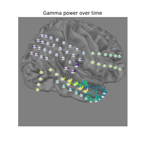
Say we want to visualize the evolution of the power in the gamma band,
instead of just plotting the average. We can use
matplotlib.animation.FuncAnimation to create an animation and apply this
to the brain figure.
# convert from a dictionary to array to plot
xy_pts = np.vstack([xy[ch] for ch in raw.info['ch_names']])
# get a colormap to color nearby points similar colors
cmap = get_cmap('viridis')
# create the figure of the brain with the electrode positions
fig, ax = plt.subplots(figsize=(5, 5))
ax.set_title('Gamma power over time', size='large')
ax.imshow(im)
ax.set_axis_off()
# normalize gamma power for plotting
gamma_power = -100 * gamma_power_t.data / gamma_power_t.data.max()
# add the time course overlaid on the positions
x_line = np.linspace(-0.025 * im.shape[0], 0.025 * im.shape[0],
gamma_power_t.data.shape[1])
for i, pos in enumerate(xy_pts):
x, y = pos
color = cmap(i / xy_pts.shape[0])
ax.plot(x_line + x, gamma_power[i] + y, linewidth=0.5, color=color)

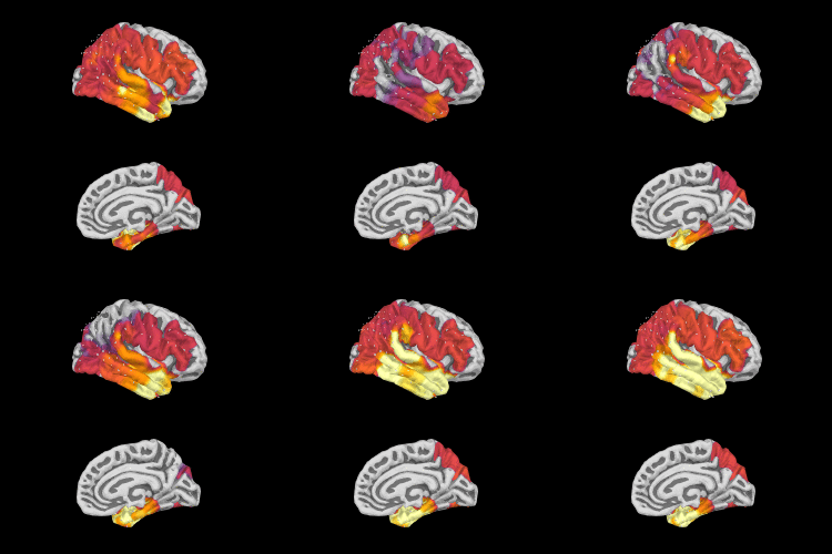
We can project gamma power from the sensor data to the nearest locations on the pial surface and visualize that:
As shown in the plot, the epileptiform activity starts in the temporal lobe,
progressing posteriorly. The seizure becomes generalized eventually, after
this example short time section. This dataset is available using
mne.datasets.epilepsy_ecog.data_path() for you to examine.
xyz_pts = np.array([dig['r'] for dig in evoked.info['dig']])
src = mne.read_source_spaces(
op.join(subjects_dir, 'fsaverage', 'bem', 'fsaverage-ico-5-src.fif'))
trans = None # identity transform
stc = mne.stc_near_sensors(gamma_power_t, trans, 'fsaverage', src=src,
mode='nearest', subjects_dir=subjects_dir,
distance=0.02)
vmin, vmid, vmax = np.percentile(gamma_power_t.data, [10, 25, 90])
clim = dict(kind='value', lims=[vmin, vmid, vmax])
brain = stc.plot(surface='pial', hemi='rh', colormap='inferno', colorbar=False,
clim=clim, views=['lat', 'med'], subjects_dir=subjects_dir,
size=(250, 250), smoothing_steps=20, time_viewer=False)
# plot electrode locations
for xyz in xyz_pts:
for subplot in (0, 1):
brain.plotter.subplot(subplot, 0)
brain._renderer.sphere(xyz * 1e3, color='white', scale=2)
# You can save a movie like the one on our documentation website with:
# brain.save_movie(time_dilation=1, interpolation='linear', framerate=12,
# time_viewer=True)
