EEG processing and Event Related Potentials (ERPs)

This tutorial shows how to perform standard ERP analyses in MNE-Python. Most of the material here is covered in other tutorials too, but for convenience the functions and methods most useful for ERP analyses are collected here, with links to other tutorials where more detailed information is given.

As usual we’ll start by importing the modules we need and loading some example data. Instead of parsing the events from the raw data’s stim channel (like we do in this tutorial), we’ll load the events from an external events file. Finally, to speed up computations so our documentation server can handle them, we’ll crop the raw data from ~4.5 minutes down to 90 seconds.

import os
import numpy as np
import matplotlib.pyplot as plt
import mne

sample_data_folder = mne.datasets.sample.data_path()
sample_data_raw_file = os.path.join(sample_data_folder, 'MEG', 'sample',
                                    'sample_audvis_filt-0-40_raw.fif')
raw = mne.io.read_raw_fif(sample_data_raw_file, preload=False)

sample_data_events_file = os.path.join(sample_data_folder, 'MEG', 'sample',
                                       'sample_audvis_filt-0-40_raw-eve.fif')
events = mne.read_events(sample_data_events_file)

raw.crop(tmax=90)  # in seconds; happens in-place
# discard events >90 seconds (not strictly necessary: avoids some warnings)
events = events[events[:, 0] <= raw.last_samp]

Out:

Opening raw data file /home/circleci/mne_data/MNE-sample-data/MEG/sample/sample_audvis_filt-0-40_raw.fif...
    Read a total of 4 projection items:
        PCA-v1 (1 x 102)  idle
        PCA-v2 (1 x 102)  idle
        PCA-v3 (1 x 102)  idle
        Average EEG reference (1 x 60)  idle
    Range : 6450 ... 48149 =     42.956 ...   320.665 secs
Ready.

The file that we loaded has already been partially processed: 3D sensor locations have been saved as part of the .fif file, the data have been low-pass filtered at 40 Hz, and a common average reference is set for the EEG channels, stored as a projector (see Creating the average reference as a projector in the Setting the EEG reference tutorial for more info about when you may want to do this). We’ll discuss how to do each of these below.

Since this is a combined EEG+MEG dataset, let’s start by restricting the data to just the EEG and EOG channels. This will cause the other projectors saved in the file (which apply only to magnetometer channels) to be removed. By looking at the measurement info we can see that we now have 59 EEG channels and 1 EOG channel.

raw.pick(['eeg', 'eog']).load_data()
raw.info

Out:

Removing projector <Projection | PCA-v1, active : False, n_channels : 102>
Removing projector <Projection | PCA-v2, active : False, n_channels : 102>
Removing projector <Projection | PCA-v3, active : False, n_channels : 102>
Reading 0 ... 13514  =      0.000 ...    90.001 secs...

Measurement date	December 03, 2002 19:01:10 GMT
Experimenter	Unknown
Participant	Unknown
Digitized points	146 points
Good channels	0 magnetometer, 0 gradiometer, and 59 EEG channels
Bad channels	EEG 053
EOG channels	EOG 061
ECG channels	Not available
Sampling frequency	150.15 Hz
Highpass	0.10 Hz
Lowpass	40.00 Hz

Channel names and types

In practice it’s quite common to have some channels labelled as EEG that are actually EOG channels. Raw objects have a set_channel_types method that you can use to change a channel that is labeled as eeg into an eog type. You can also rename channels using the rename_channels method. Detailed examples of both of these methods can be found in the tutorial The Raw data structure: continuous data. In this data the channel types are all correct already, so for now we’ll just rename the channels to remove a space and a leading zero in the channel names, and convert to lowercase:

channel_renaming_dict = {name: name.replace(' 0', '').lower()
                         for name in raw.ch_names}
_ = raw.rename_channels(channel_renaming_dict)  # happens in-place

Channel locations

The tutorial Working with sensor locations describes MNE-Python’s handling of sensor positions in great detail. To briefly summarize: MNE-Python distinguishes montages (which contain sensor positions in 3D: x, y, z, in meters) from layouts (which define 2D arrangements of sensors for plotting approximate overhead diagrams of sensor positions). Additionally, montages may specify idealized sensor positions (based on, e.g., an idealized spherical headshape model) or they may contain realistic sensor positions obtained by digitizing the 3D locations of the sensors when placed on the actual subject’s head.

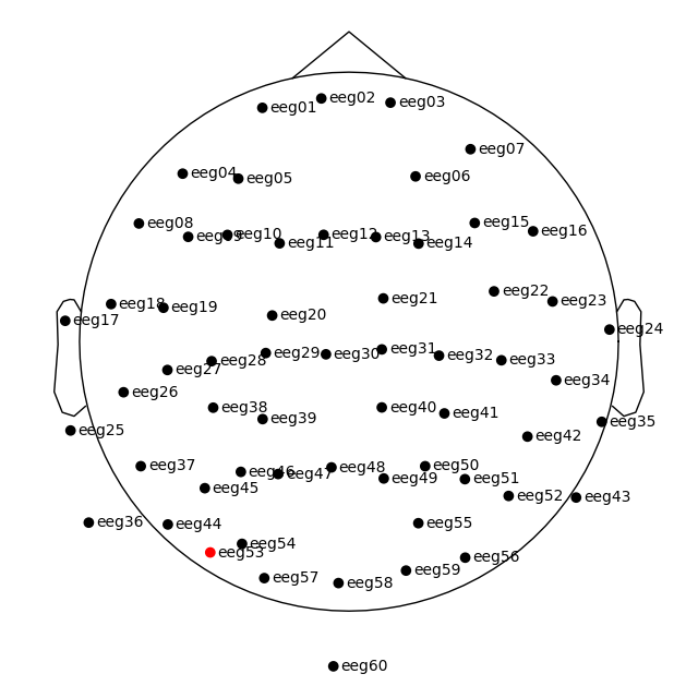
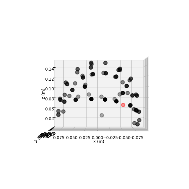
This dataset has realistic digitized 3D sensor locations saved as part of the .fif file, so we can view the sensor locations in 2D or 3D using the plot_sensors method:

raw.plot_sensors(show_names=True)
fig = raw.plot_sensors('3d')

• 
• 

If you’re working with a standard montage like the 10-20 system, you can add sensor locations to the data like this: raw.set_montage('standard_1020'). See Working with sensor locations for info on what other standard montages are built-in to MNE-Python.

If you have digitized realistic sensor locations, there are dedicated functions for loading those digitization files into MNE-Python; see Reading sensor digitization files for discussion and Supported formats for digitized 3D locations for a list of supported formats. Once loaded, the digitized sensor locations can be added to the data by passing the loaded montage object to raw.set_montage().

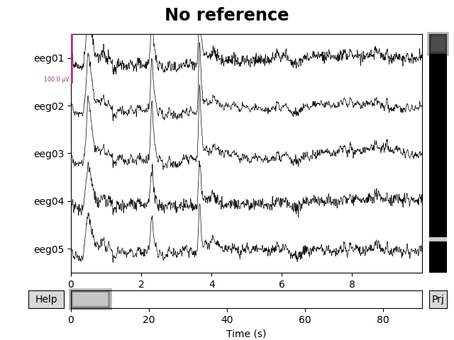
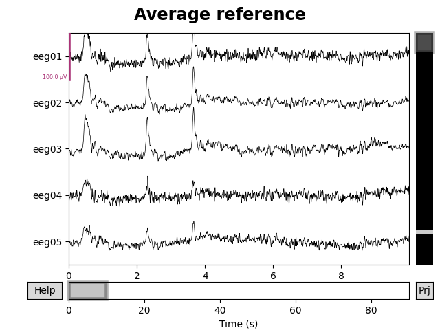
Setting the EEG reference

As mentioned above, this data already has an EEG common average reference added as a projector. We can view the effect of this on the raw data by plotting with and without the projector applied:

for proj in (False, True):
    fig = raw.plot(n_channels=5, proj=proj, scalings=dict(eeg=50e-6))
    fig.subplots_adjust(top=0.9)  # make room for title
    ref = 'Average' if proj else 'No'
    fig.suptitle(f'{ref} reference', size='xx-large', weight='bold')

• 
• 

The referencing scheme can be changed with the function mne.set_eeg_reference (which by default operates on a copy of the data) or the raw.set_eeg_reference() method (which always modifies the data in-place). The tutorial Setting the EEG reference shows several examples of this.

Filtering

MNE-Python has extensive support for different ways of filtering data. For a general discussion of filter characteristics and MNE-Python defaults, see Background information on filtering. For practical examples of how to apply filters to your data, see Filtering and resampling data. Here, we’ll apply a simple high-pass filter for illustration:

raw.filter(l_freq=0.1, h_freq=None)

Out:

Filtering raw data in 1 contiguous segment
Setting up high-pass filter at 0.1 Hz

FIR filter parameters
---------------------
Designing a one-pass, zero-phase, non-causal highpass filter:
- Windowed time-domain design (firwin) method
- Hamming window with 0.0194 passband ripple and 53 dB stopband attenuation
- Lower passband edge: 0.10
- Lower transition bandwidth: 0.10 Hz (-6 dB cutoff frequency: 0.05 Hz)
- Filter length: 4957 samples (33.013 sec)

Measurement date	December 03, 2002 19:01:10 GMT
Experimenter	Unknown
Participant	Unknown
Digitized points	146 points
Good channels	0 magnetometer, 0 gradiometer, and 59 EEG channels
Bad channels	eeg53
EOG channels	eog61
ECG channels	Not available
Sampling frequency	150.15 Hz
Highpass	0.10 Hz
Lowpass	40.00 Hz
Filenames	sample_audvis_filt-0-40_raw.fif
Duration	00:01:30 (HH:MM:SS)

Evoked responses: epoching and averaging

The general process for extracting evoked responses from continuous data is to use the Epochs constructor, and then average the resulting epochs to create an Evoked object. In MNE-Python, events are represented as a NumPy array of sample numbers and integer event codes. The event codes are stored in the last column of the events array:

np.unique(events[:, -1])

The Working with events tutorial discusses event arrays in more detail. Integer event codes are mapped to more descriptive text using a Python dictionary usually called event_id. This mapping is determined by your experiment code (i.e., it reflects which event codes you chose to use to represent different experimental events or conditions). For the Sample data has the following mapping:

event_dict = {'auditory/left': 1, 'auditory/right': 2, 'visual/left': 3,
              'visual/right': 4, 'face': 5, 'buttonpress': 32}

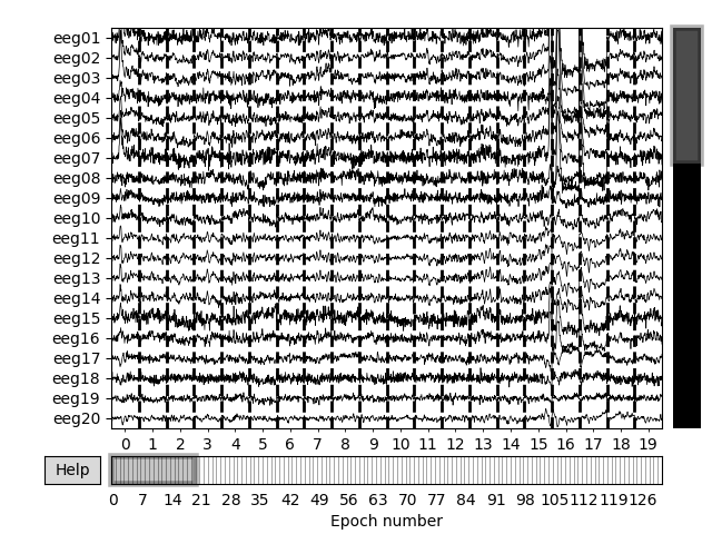
Now we can extract epochs from the continuous data. An interactive plot allows you to click on epochs to mark them as “bad” and drop them from the analysis (it is not interactive on the documentation website, but will be when you run epochs.plot() in a Python console).

epochs = mne.Epochs(raw, events, event_id=event_dict, tmin=-0.3, tmax=0.7,
                    preload=True)
fig = epochs.plot()

Out:

Not setting metadata
Not setting metadata
132 matching events found
Setting baseline interval to [-0.2996928197375818, 0.0] sec
Applying baseline correction (mode: mean)
Created an SSP operator (subspace dimension = 1)
1 projection items activated
Loading data for 132 events and 151 original time points ...
1 bad epochs dropped

It is also possible to automatically drop epochs, when first creating them or later on, by providing maximum peak-to-peak signal value thresholds (pass to the Epochs constructor as the reject parameter; see Rejecting Epochs based on channel amplitude for details). You can also do this after the epochs are already created, using the drop_bad method:

reject_criteria = dict(eeg=100e-6,  # 100 µV
                       eog=200e-6)  # 200 µV
_ = epochs.drop_bad(reject=reject_criteria)

Out:

    Rejecting  epoch based on EEG : ['eeg03']
    Rejecting  epoch based on EEG : ['eeg01', 'eeg02', 'eeg03', 'eeg04', 'eeg06', 'eeg07']
    Rejecting  epoch based on EEG : ['eeg01', 'eeg02', 'eeg03', 'eeg04', 'eeg06', 'eeg07']
    Rejecting  epoch based on EEG : ['eeg01', 'eeg02', 'eeg03', 'eeg04', 'eeg06', 'eeg07']
    Rejecting  epoch based on EEG : ['eeg01', 'eeg02', 'eeg03', 'eeg07']
    Rejecting  epoch based on EEG : ['eeg01', 'eeg02', 'eeg03', 'eeg07']
    Rejecting  epoch based on EEG : ['eeg01']
    Rejecting  epoch based on EEG : ['eeg03', 'eeg07']
    Rejecting  epoch based on EEG : ['eeg03', 'eeg07']
    Rejecting  epoch based on EEG : ['eeg07']
    Rejecting  epoch based on EEG : ['eeg03', 'eeg07']
    Rejecting  epoch based on EEG : ['eeg03', 'eeg07']
    Rejecting  epoch based on EEG : ['eeg07']
    Rejecting  epoch based on EEG : ['eeg07']
    Rejecting  epoch based on EEG : ['eeg03']
    Rejecting  epoch based on EEG : ['eeg25']
    Rejecting  epoch based on EEG : ['eeg25']
17 bad epochs dropped

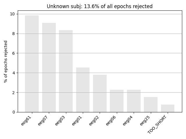
Next we generate a barplot of which channels contributed most to epochs getting rejected. If one channel is responsible for lots of epoch rejections, it may be worthwhile to mark that channel as “bad” in the Raw object and then re-run epoching (fewer channels w/ more good epochs may be preferable to keeping all channels but losing many epochs). See Handling bad channels for more info.

epochs.plot_drop_log()

Another way in which epochs can be automatically dropped is if the Raw object they’re extracted from contains annotations that begin with either bad or edge (“edge” annotations are automatically inserted when concatenating two separate Raw objects together). See Rejecting bad data spans for more information about annotation-based epoch rejection.

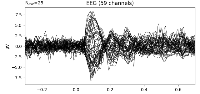
Now that we’ve dropped the bad epochs, let’s look at our evoked responses for some conditions we care about. Here the average method will create and Evoked object, which we can then plot. Notice that weselect which condition we want to average using the square-bracket indexing (like a dictionary); that returns a smaller epochs object containing just the epochs from that condition, to which we then apply the average method:

l_aud = epochs['auditory/left'].average()
l_vis = epochs['visual/left'].average()

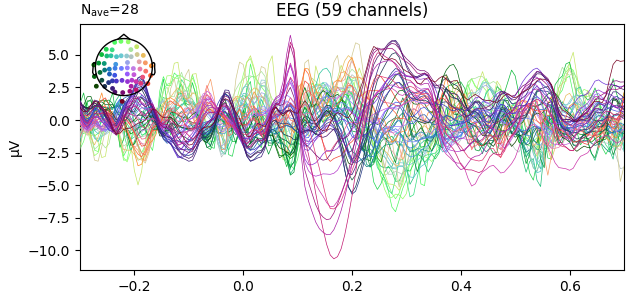
These Evoked objects have their own interactive plotting method (though again, it won’t be interactive on the documentation website): click-dragging a span of time will generate a scalp field topography for that time span. Here we also demonstrate built-in color-coding the channel traces by location:

fig1 = l_aud.plot()
fig2 = l_vis.plot(spatial_colors=True)

• 
• 

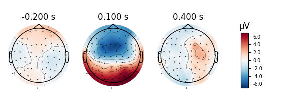
Scalp topographies can also be obtained non-interactively with the plot_topomap method. Here we display topomaps of the average field in 50 ms time windows centered at -200 ms, 100 ms, and 400 ms.

l_aud.plot_topomap(times=[-0.2, 0.1, 0.4], average=0.05)

Considerable customization of these plots is possible, see the docstring of plot_topomap for details.

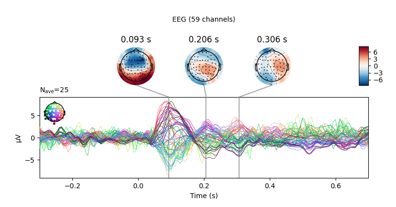
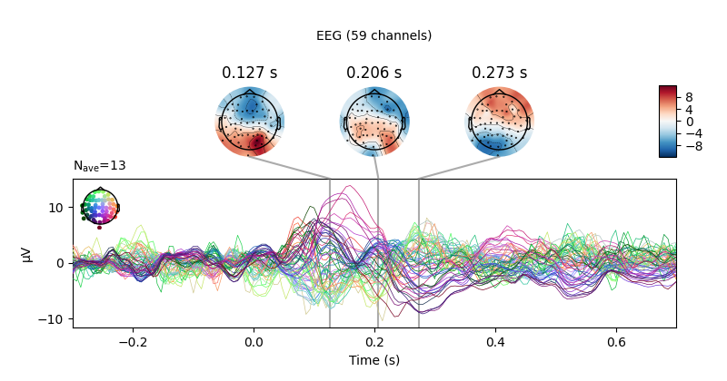
There is also a built-in method for combining “butterfly” plots of the signals with scalp topographies, called plot_joint. Like plot_topomap you can specify times for the scalp topographies or you can let the method choose times automatically, as is done here:

l_aud.plot_joint()

Out:

Projections have already been applied. Setting proj attribute to True.

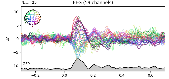
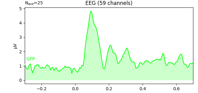
Global field power (GFP)

Global field power 123 is, generally speaking, a measure of agreement of the signals picked up by all sensors across the entire scalp: if all sensors have the same value at a given time point, the GFP will be zero at that time point; if the signals differ, the GFP will be non-zero at that time point. GFP peaks may reflect “interesting” brain activity, warranting further investigation. Mathematically, the GFP is the population standard deviation across all sensors, calculated separately for every time point.

You can plot the GFP using evoked.plot(gfp=True). The GFP trace will be black if spatial_colors=True and green otherwise. The EEG reference does not affect the GFP:

for evk in (l_aud, l_vis):
    evk.plot(gfp=True, spatial_colors=True, ylim=dict(eeg=[-12, 12]))

• 
• 

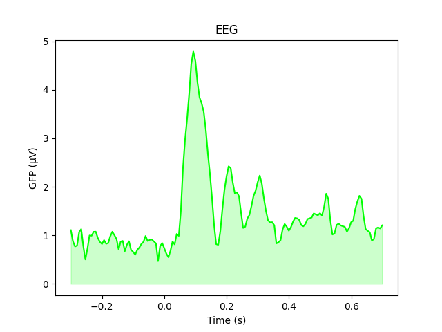
To plot the GFP by itself you can pass gfp='only' (this makes it easier to read off the GFP data values, because the scale is aligned):

l_aud.plot(gfp='only')

As stated above, the GFP is the population standard deviation of the signal across channels. To compute it manually, we can leverage the fact that evoked.data is a NumPy array, and verify by plotting it using matplotlib commands:

gfp = l_aud.data.std(axis=0, ddof=0)

# Reproducing the MNE-Python plot style seen above
fig, ax = plt.subplots()
ax.plot(l_aud.times, gfp * 1e6, color='lime')
ax.fill_between(l_aud.times, gfp * 1e6, color='lime', alpha=0.2)
ax.set(xlabel='Time (s)', ylabel='GFP (µV)', title='EEG')

Analyzing regions of interest (ROIs): averaging across channels

Since our sample data is responses to left and right auditory and visual stimuli, we may want to compare left versus right ROIs. To average across channels in a region of interest, we first find the channel indices we want. Looking back at the 2D sensor plot above, we might choose the following for left and right ROIs:

left = ['eeg17', 'eeg18', 'eeg25', 'eeg26']
right = ['eeg23', 'eeg24', 'eeg34', 'eeg35']

left_ix = mne.pick_channels(l_aud.info['ch_names'], include=left)
right_ix = mne.pick_channels(l_aud.info['ch_names'], include=right)

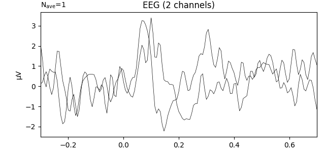
Now we can create a new Evoked with 2 virtual channels (one for each ROI):

roi_dict = dict(left_ROI=left_ix, right_ROI=right_ix)
roi_evoked = mne.channels.combine_channels(l_aud, roi_dict, method='mean')
print(roi_evoked.info['ch_names'])
roi_evoked.plot()

Out:

['left_ROI', 'right_ROI']

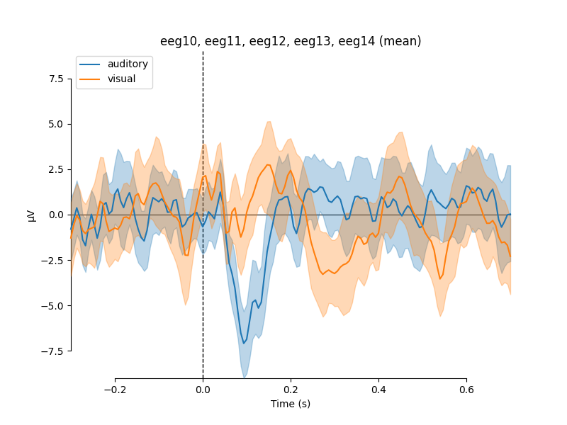
Comparing conditions

If we wanted to compare our auditory and visual stimuli, a useful function is mne.viz.plot_compare_evokeds. By default this will combine all channels in each evoked object using global field power (or RMS for MEG channels); here instead we specify to combine by averaging, and restrict it to a subset of channels by passing picks:

evokeds = dict(auditory=l_aud, visual=l_vis)
picks = [f'eeg{n}' for n in range(10, 15)]
mne.viz.plot_compare_evokeds(evokeds, picks=picks, combine='mean')

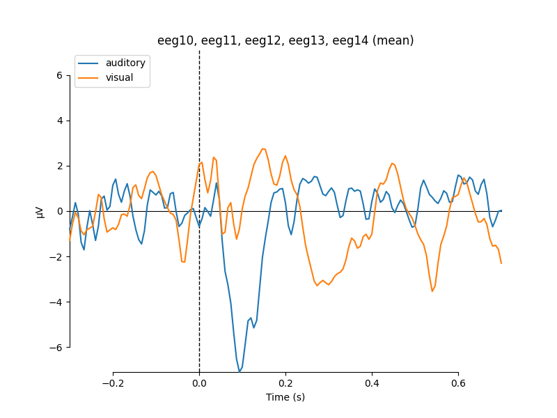
Out:

combining channels using "mean"
combining channels using "mean"

We can also easily get confidence intervals by treating each epoch as a separate observation using the iter_evoked method. A confidence interval across subjects could also be obtained, by passing a list of Evoked objects (one per subject) to the plot_compare_evokeds function.

evokeds = dict(auditory=list(epochs['auditory/left'].iter_evoked()),
               visual=list(epochs['visual/left'].iter_evoked()))
mne.viz.plot_compare_evokeds(evokeds, combine='mean', picks=picks)

Out:

combining channels using "mean"
combining channels using "mean"

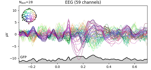
We can also compare conditions by subtracting one Evoked object from another using the mne.combine_evoked function (this function also allows pooling of epochs without subtraction).

aud_minus_vis = mne.combine_evoked([l_aud, l_vis], weights=[1, -1])
aud_minus_vis.plot_joint()

Out:

Projections have already been applied. Setting proj attribute to True.

Warning

The code above yields an equal-weighted difference. If you have imbalanced trial numbers, you might want to equalize the number of events per condition first by using epochs.equalize_event_counts() before averaging.

Grand averages

To compute grand averages across conditions (or subjects), you can pass a list of Evoked objects to mne.grand_average. The result is another Evoked object.

grand_average = mne.grand_average([l_aud, l_vis])
print(grand_average)

Out:

Interpolating bad channels
    Automatic origin fit: head of radius 91.0 mm
Computing interpolation matrix from 59 sensor positions
Interpolating 1 sensors
Interpolating bad channels
    Automatic origin fit: head of radius 91.0 mm
Computing interpolation matrix from 59 sensor positions
Interpolating 1 sensors
Identifying common channels ...
<Evoked | 'Grand average (n = 2)' (average, N=2), -0.29969 – 0.69928 sec, baseline -0.299693 – 0 sec, 60 ch, ~3.0 MB>

For combining conditions it is also possible to make use of HED tags in the condition names when selecting which epochs to average. For example, we have the condition names:

list(event_dict)

We can select the auditory conditions (left and right together) by passing:

epochs['auditory'].average()

see Subselecting epochs for details.

The tutorials The Epochs data structure: discontinuous data and The Evoked data structure: evoked/averaged data have many more details about working with the Epochs and Evoked classes.

References

1

Dietrich Lehmann and Wolfgang Skrandies. Reference-free identification of components of checkerboard-evoked multichannel potential fields. Electroencephalography and Clinical Neurophysiology, 48(6):609–621, 1980. doi:10.1016/0013-4694(80)90419-8.

2

Dietrich Lehmann and Wolfgang Skrandies. Spatial analysis of evoked potentials in man—a review. Progress in Neurobiology, 23(3):227–250, 1984. doi:10.1016/0301-0082(84)90003-0.

3

Micah M. Murray, Denis Brunet, and Christoph M. Michel. Topographic ERP analyses: A step-by-step tutorial review. Brain Topography, 20(4):249–264, 2008. doi:10.1007/s10548-008-0054-5.

Estimated memory usage: 8 MB

Visualizing Evoked data Plotting whitened data