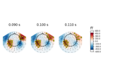
mne.viz.plot_topomap#
- mne.viz.plot_topomap(data, pos, *, ch_type='eeg', sensors=True, show_names=None, names=None, mask=None, mask_params=None, contours=6, outlines='head', sphere=None, image_interp='cubic', extrapolate='auto', border='mean', res=64, size=1, cmap=None, vlim=(None, None), vmin=None, vmax=None, cnorm=None, axes=None, show=True, onselect=None)[source]#
Plot a topographic map as image.
- Parameters:
- data
array, shape (n_chan,) The data values to plot.
- pos
array, shape (n_channels, 2) | instance ofInfo Location information for the channels. If an array, should provide the x and y coordinates for plotting the channels in 2D. If an
Infoobject it must contain only one channel type and exactlylen(data)channels; the x/y coordinates will be inferred from the montage in theInfoobject.- ch_type‘mag’ | ‘grad’ | ‘planar1’ | ‘planar2’ | ‘eeg’ |
None The channel type to plot. For
'grad', the gradiometers are collected in pairs and the RMS for each pair is plotted. IfNonethe first available channel type from order shown above is used. Defaults toNone.New in version 0.21.
- sensors
bool|str Whether to add markers for sensor locations. If
str, should be a valid matplotlib format string (e.g.,'r+'for red plusses, see the Notes section ofplot()). IfTrue(the default), black circles will be used.- show_names
bool|callable() If
True, show channel names next to each sensor marker. If callable, channel names will be formatted using the callable; e.g., to delete the prefix ‘MEG ‘ from all channel names, pass the functionlambda x: x.replace('MEG ', ''). Ifmaskis notNone, only non-masked sensor names will be shown.Deprecated since version v1.2: The
show_namesparameter will be removed in version 1.3. Please use thenamesparameter instead.- names
None|list Labels for the sensors. If a
list, labels should correspond to the order of channels indata. IfNone(default), no channel names are plotted.- mask
ndarrayofbool, shape (n_channels,) |None Array indicating channel(s) to highlight with a distinct plotting style. Array elements set to
Truewill be plotted with the parameters given inmask_params. Defaults toNone, equivalent to an array of allFalseelements.- mask_params
dict|None Additional plotting parameters for plotting significant sensors. Default (None) equals:
dict(marker='o', markerfacecolor='w', markeredgecolor='k',
        linewidth=0, markersize=4)
- contours
int| array_like The number of contour lines to draw. If
0, no contours will be drawn. If a positive integer, that number of contour levels are chosen using the matplotlib tick locator (may sometimes be inaccurate, use array for accuracy). If array-like, the array values are used as the contour levels. The values should be in µV for EEG, fT for magnetometers and fT/m for gradiometers. Ifcolorbar=True, the colorbar will have ticks corresponding to the contour levels. Default is6.- outlines‘head’ | ‘skirt’ |
dict|None The outlines to be drawn. If ‘head’, the default head scheme will be drawn. If ‘skirt’ the head scheme will be drawn, but sensors are allowed to be plotted outside of the head circle. If dict, each key refers to a tuple of x and y positions, the values in ‘mask_pos’ will serve as image mask. Alternatively, a matplotlib patch object can be passed for advanced masking options, either directly or as a function that returns patches (required for multi-axis plots). If None, nothing will be drawn. Defaults to ‘head’.
Deprecated since version v1.2: The
outlines='skirt'option is no longer supported and will raise an error starting in version 1.3. Passoutlines='head', sphere='eeglab'for similar behavior.- sphere
float| array_like | instance ofConductorModel|None| ‘auto’ | ‘eeglab’ The sphere parameters to use for the head outline. Can be array-like of shape (4,) to give the X/Y/Z origin and radius in meters, or a single float to give just the radius (origin assumed 0, 0, 0). Can also be an instance of a spherical
ConductorModelto use the origin and radius from that object. If'auto'the sphere is fit to digitization points. If'eeglab'the head circle is defined by EEG electrodes'Fpz','Oz','T7', and'T8'(if'Fpz'is not present, it will be approximated from the coordinates of'Oz').None(the default) is equivalent to'auto'when enough extra digitization points are available, and (0, 0, 0, 0.095) otherwise.New in version 0.20.
Changed in version 1.1: Added
'eeglab'option.- image_interp
str The image interpolation to be used. Options are
'cubic'(default) to usescipy.interpolate.CloughTocher2DInterpolator,'nearest'to usescipy.spatial.Voronoior'linear'to usescipy.interpolate.LinearNDInterpolator.- extrapolate
str Options:
'box'Extrapolate to four points placed to form a square encompassing all data points, where each side of the square is three times the range of the data in the respective dimension.
'local'(default for MEG sensors)Extrapolate only to nearby points (approximately to points closer than median inter-electrode distance). This will also set the mask to be polygonal based on the convex hull of the sensors.
'head'(default for non-MEG sensors)Extrapolate out to the edges of the clipping circle. This will be on the head circle when the sensors are contained within the head circle, but it can extend beyond the head when sensors are plotted outside the head circle.
Changed in version 0.21:
The default was changed to
'local'for MEG sensors.'local'was changed to use a convex hull mask'head'was changed to extrapolate out to the clipping circle.
New in version 0.18.
- border
float| ‘mean’ Value to extrapolate to on the topomap borders. If
'mean'(default), then each extrapolated point has the average value of its neighbours.New in version 0.20.
- res
int The resolution of the topomap image (number of pixels along each side).
- size
float Side length of each subplot in inches.
- cmapmatplotlib colormap |
None Colormap to use. If None, ‘Reds’ is used for all positive data, otherwise defaults to ‘RdBu_r’.
- vlim
tupleof length 2 Colormap limits to use. If a
tupleof floats, specifies the lower and upper bounds of the colormap (in that order); providingNonefor either entry will set the corresponding boundary at the min/max of the data. Defaults to(None, None).New in version 1.2.
- vmin, vmax
float|callable()|None Lower and upper bounds of the colormap, in the same units as the data. If
vminandvmaxare bothNone, they are set at ± the maximum absolute value of the data (yielding a colormap with midpoint at 0). If only one ofvmin,vmaxisNone, will usemin(data)ormax(data), respectively. If callable, should accept aNumPy arrayof data and return a float.Deprecated since version v1.2: The
vminandvmaxparameters will be removed in version 1.3. Please use thevlimparameter instead.- cnorm
matplotlib.colors.Normalize|None How to normalize the colormap. If
None, standard linear normalization is performed. If notNone,vminandvmaxwill be ignored. See Matplotlib docs for more details on colormap normalization, and the ERDs example for an example of its use.New in version 0.24.
- axesinstance of
Axes|None The axes to plot to. If
None, a newFigurewill be created. Default isNone.Changed in version 1.2: If
axes=None, a newFigureis created instead of plotting into the current axes.- show
bool Show the figure if
True.- onselect
callable()|None A function to be called when the user selects a set of channels by click-dragging (uses a matplotlib
RectangleSelector). IfNoneinteractive channel selection is disabled. Defaults toNone.
- data
- Returns:
- im
matplotlib.image.AxesImage The interpolated data.
- cn
matplotlib.contour.ContourSet The fieldlines.
- im
Examples using mne.viz.plot_topomap#
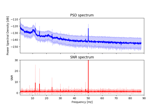
Frequency-tagging: Basic analysis of an SSVEP/vSSR dataset