Note
Go to the end to download the full example code
Preprocessing optically pumped magnetometer (OPM) MEG data#
This tutorial covers preprocessing steps that are specific to OPM MEG data. OPMs use a different sensing technology than traditional SQUID MEG systems, which leads to several important differences for analysis:
They are sensitive to DC magnetic fields
Sensor layouts can vary by participant and recording session due to flexible sensor placement
Devices are typically not fixed in place, so the position of the sensors relative to the room (and through the DC fields) can change over time
We will cover some of these considerations here by processing the UCL OPM auditory dataset [1]
import matplotlib.pyplot as plt
import numpy as np

import mne

opm_data_folder = mne.datasets.ucl_opm_auditory.data_path()
opm_file = (
    opm_data_folder
    / "sub-002"
    / "ses-001"
    / "meg"
    / "sub-002_ses-001_task-aef_run-001_meg.bin"
)
# For now we are going to assume the device and head coordinate frames are
# identical (even though this is incorrect), so we pass verbose='error' for now
raw = mne.io.read_raw_fil(opm_file, verbose="error")
raw.crop(120, 210).load_data()  # crop for speed
Reading 0 ... 540000 = 0.000 ... 90.000 secs...
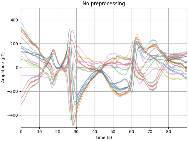
Examining raw data#
First, let’s look at the raw data, noting that there are large fluctuations in the sub 1 Hz band. In some cases the range of fields a single channel reports is as much as 600 pT across this experiment.
picks = mne.pick_types(raw.info, meg=True)

amp_scale = 1e12  # T->pT
stop = len(raw.times) - 300
step = 300
data_ds, time_ds = raw[picks[::5], :stop]
data_ds, time_ds = data_ds[:, ::step] * amp_scale, time_ds[::step]

fig, ax = plt.subplots(constrained_layout=True)
plot_kwargs = dict(lw=1, alpha=0.5)
ax.plot(time_ds, data_ds.T - np.mean(data_ds, axis=1), **plot_kwargs)
ax.grid(True)
set_kwargs = dict(
    ylim=(-500, 500), xlim=time_ds[[0, -1]], xlabel="Time (s)", ylabel="Amplitude (pT)"
)
ax.set(title="No preprocessing", **set_kwargs)
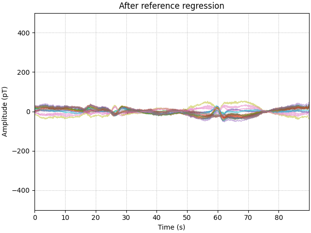
Denoising: Regressing via reference sensors#
The simplest method for reducing low frequency drift in the data is to use a set of reference sensors away from the scalp, which only sample the ambient fields in the room. An advantage of this method is that no prior knowldge of the locations of the sensors is required. However, it assumes that the reference sensors experience the same interference as scalp recordings.
To do this in our current dataset, we require a bit of housekeeping. There are a set of channels beginning with the name “Flux” which do not contain any evironmental data, these need to be set to as bad channels. Another channel – G2-17-TAN – will also be set to bad.
For now we are only interested in removing artefacts seen below 5 Hz, so we initially low-pass filter the good reference channels in this dataset prior to regression
Looking at the processed data, we see there has been a large reduction in the low frequency drift, but there are still periods where the drift has not been entirely removed. The likely cause of this is that the spatial profile of the interference is dynamic, so performing a single regression over the entire experiment is not the most effective approach.
# set flux channels to bad
bad_picks = mne.pick_channels_regexp(raw.ch_names, regexp="Flux.")
raw.info["bads"].extend([raw.ch_names[ii] for ii in bad_picks])
raw.info["bads"].extend(["G2-17-TAN"])

# compute the PSD for later using 1 Hz resolution
psd_kwargs = dict(fmax=20, n_fft=int(round(raw.info["sfreq"])))
psd_pre = raw.compute_psd(**psd_kwargs)

# filter and regress
raw.filter(None, 5, picks="ref_meg")
regress = mne.preprocessing.EOGRegression(picks, picks_artifact="ref_meg")
regress.fit(raw)
regress.apply(raw, copy=False)

# plot
data_ds, _ = raw[picks[::5], :stop]
data_ds = data_ds[:, ::step] * amp_scale

fig, ax = plt.subplots(constrained_layout=True)
ax.plot(time_ds, data_ds.T - np.mean(data_ds, axis=1), **plot_kwargs)
ax.grid(True, ls=":")
ax.set(title="After reference regression", **set_kwargs)

# compute the psd of the regressed data
psd_post_reg = raw.compute_psd(**psd_kwargs)
Effective window size : 1.000 (s)
Filtering a subset of channels. The highpass and lowpass values in the measurement info will not be updated.
Filtering raw data in 1 contiguous segment
Setting up low-pass filter at 5 Hz

FIR filter parameters
---------------------
Designing a one-pass, zero-phase, non-causal lowpass filter:
- Windowed time-domain design (firwin) method
- Hamming window with 0.0194 passband ripple and 53 dB stopband attenuation
- Upper passband edge: 5.00 Hz
- Upper transition bandwidth: 2.00 Hz (-6 dB cutoff frequency: 6.00 Hz)
- Filter length: 9901 samples (1.650 s)

[Parallel(n_jobs=1)]: Using backend SequentialBackend with 1 concurrent workers.
[Parallel(n_jobs=1)]: Done   1 out of   1 | elapsed:    0.0s remaining:    0.0s
[Parallel(n_jobs=1)]: Done   2 out of   2 | elapsed:    0.0s remaining:    0.0s
[Parallel(n_jobs=1)]: Done   3 out of   3 | elapsed:    0.1s remaining:    0.0s
[Parallel(n_jobs=1)]: Done   4 out of   4 | elapsed:    0.1s remaining:    0.0s
[Parallel(n_jobs=1)]: Done   8 out of   8 | elapsed:    0.2s finished
No projector specified for this dataset. Please consider the method self.add_proj.
No projector specified for this dataset. Please consider the method self.add_proj.
Effective window size : 1.000 (s)
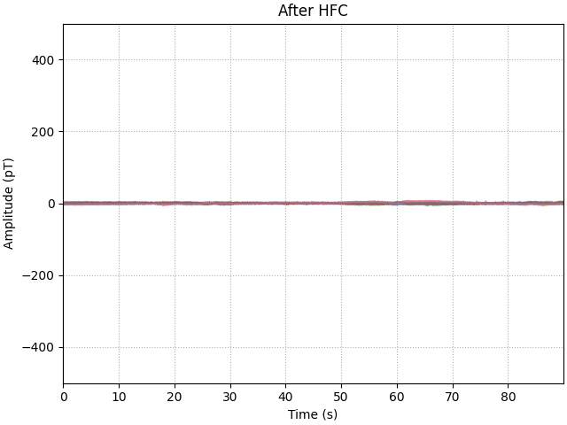
Denoising: Regressing via homogeneous field correction#
Regression of a reference channel is a start, but in this instance assumes the relatiship between the references and a given sensor on the head as constant. However this becomes less accurate when the reference is not moving but the subject is. An alternative method, Homogeneous Field Correction (HFC) only requires that the sensors on the helmet stationary relative to each other. Which in a well-designed rigid helmet is the case.
# include gradients by setting order to 2, set to 1 for homgenous components
projs = mne.preprocessing.compute_proj_hfc(raw.info, order=2)
raw.add_proj(projs).apply_proj(verbose="error")

# plot
data_ds, _ = raw[picks[::5], :stop]
data_ds = data_ds[:, ::step] * amp_scale

fig, ax = plt.subplots(constrained_layout=True)
ax.plot(time_ds, data_ds.T - np.mean(data_ds, axis=1), **plot_kwargs)
ax.grid(True, ls=":")
ax.set(title="After HFC", **set_kwargs)

# compute the psd of the regressed data
psd_post_hfc = raw.compute_psd(**psd_kwargs)
8 projection items deactivated
Effective window size : 1.000 (s)
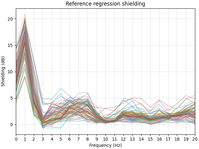
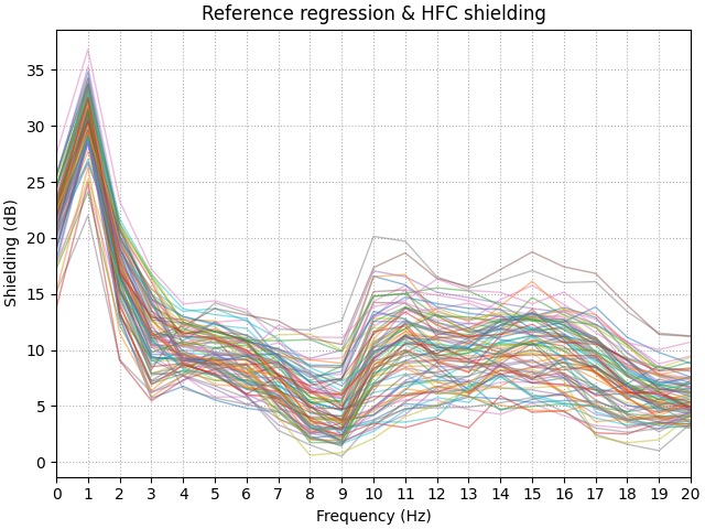
Comparing denoising methods#
Differing denoising methods will have differing levels of performance across different parts of the spectrum. One way to evaluate the performance of a denoising step is to calculate the power spectrum of the dataset before and after processing. We will use metric called the shielding factor to summarise the values. Positive shielding factors indicate a reduction in power, whilst negative means in increase.
We see that reference regression does a good job in reducing low frequency drift up to ~2 Hz, with 20 dB of shielding. But rapidly drops off due to low pass filtering the reference signal at 5 Hz. We also can see that this method is also introducing additional interference at 3 Hz.
HFC improves on the low frequency shielding (up to 32 dB). Also this method is not frequency-specific so we observe broadband interference reduction.
shielding = 10 * np.log10(psd_pre[:] / psd_post_reg[:])

fig, ax = plt.subplots(constrained_layout=True)
ax.plot(psd_post_reg.freqs, shielding.T, **plot_kwargs)
ax.grid(True, ls=":")
ax.set(xticks=psd_post_reg.freqs)
ax.set(
    xlim=(0, 20),
    title="Reference regression shielding",
    xlabel="Frequency (Hz)",
    ylabel="Shielding (dB)",
)


shielding = 10 * np.log10(psd_pre[:] / psd_post_hfc[:])

fig, ax = plt.subplots(constrained_layout=True)
ax.plot(psd_post_hfc.freqs, shielding.T, **plot_kwargs)
ax.grid(True, ls=":")
ax.set(xticks=psd_post_hfc.freqs)
ax.set(
    xlim=(0, 20),
    title="Reference regression & HFC shielding",
    xlabel="Frequency (Hz)",
    ylabel="Shielding (dB)",
)
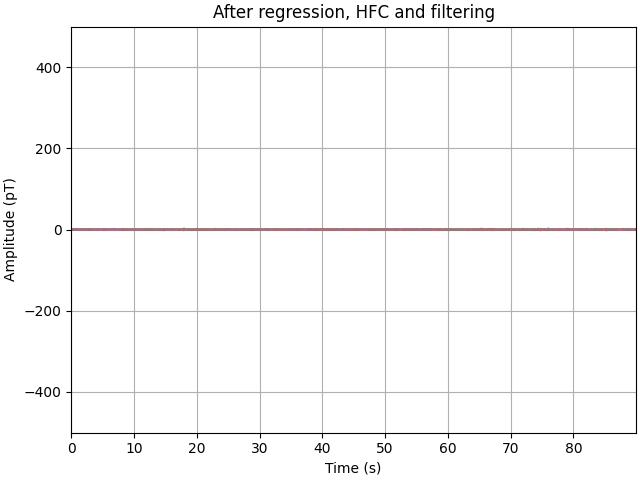
Filtering nuisance signals#
Having regressed much of the high-amplitude, low-frequency interference, we can now look to filtering the remnant nuisance signals. The motivation for filtering after regression (rather than before) is to minimise any filter artefacts generated when removing such high-amplitude interfece (compared to the neural signals we are interested in).
We are going to remove the 50 Hz mains signal with a notch filter, followed by a bandpass filter between 2 and 40 Hz. From here it becomes clear that the variance in our signal has been reduced from 100s of pT to 10s of pT instead.
# notch
raw.notch_filter(np.arange(50, 251, 50), notch_widths=4)
# bandpass
raw.filter(2, 40, picks="meg")
# plot
data_ds, _ = raw[picks[::5], :stop]
data_ds = data_ds[:, ::step] * amp_scale
fig, ax = plt.subplots(constrained_layout=True)
plot_kwargs = dict(lw=1, alpha=0.5)
ax.plot(time_ds, data_ds.T - np.mean(data_ds, axis=1), **plot_kwargs)
ax.grid(True)
set_kwargs = dict(
    ylim=(-500, 500), xlim=time_ds[[0, -1]], xlabel="Time (s)", ylabel="Amplitude (pT)"
)
ax.set(title="After regression, HFC and filtering", **set_kwargs)
Filtering raw data in 1 contiguous segment
Setting up band-stop filter

FIR filter parameters
---------------------
Designing a one-pass, zero-phase, non-causal bandstop filter:
- Windowed time-domain design (firwin) method
- Hamming window with 0.0194 passband ripple and 53 dB stopband attenuation
- Lower transition bandwidth: 0.50 Hz
- Upper transition bandwidth: 0.50 Hz
- Filter length: 39601 samples (6.600 s)

[Parallel(n_jobs=1)]: Using backend SequentialBackend with 1 concurrent workers.
[Parallel(n_jobs=1)]: Done   1 out of   1 | elapsed:    0.0s remaining:    0.0s
[Parallel(n_jobs=1)]: Done   2 out of   2 | elapsed:    0.1s remaining:    0.0s
[Parallel(n_jobs=1)]: Done   3 out of   3 | elapsed:    0.1s remaining:    0.0s
[Parallel(n_jobs=1)]: Done   4 out of   4 | elapsed:    0.1s remaining:    0.0s
[Parallel(n_jobs=1)]: Done  94 out of  94 | elapsed:    3.0s finished
Filtering a subset of channels. The highpass and lowpass values in the measurement info will not be updated.
Filtering raw data in 1 contiguous segment
Setting up band-pass filter from 2 - 40 Hz

FIR filter parameters
---------------------
Designing a one-pass, zero-phase, non-causal bandpass filter:
- Windowed time-domain design (firwin) method
- Hamming window with 0.0194 passband ripple and 53 dB stopband attenuation
- Lower passband edge: 2.00
- Lower transition bandwidth: 2.00 Hz (-6 dB cutoff frequency: 1.00 Hz)
- Upper passband edge: 40.00 Hz
- Upper transition bandwidth: 10.00 Hz (-6 dB cutoff frequency: 45.00 Hz)
- Filter length: 9901 samples (1.650 s)

[Parallel(n_jobs=1)]: Using backend SequentialBackend with 1 concurrent workers.
[Parallel(n_jobs=1)]: Done   1 out of   1 | elapsed:    0.0s remaining:    0.0s
[Parallel(n_jobs=1)]: Done   2 out of   2 | elapsed:    0.0s remaining:    0.0s
[Parallel(n_jobs=1)]: Done   3 out of   3 | elapsed:    0.1s remaining:    0.0s
[Parallel(n_jobs=1)]: Done   4 out of   4 | elapsed:    0.1s remaining:    0.0s
[Parallel(n_jobs=1)]: Done  86 out of  86 | elapsed:    1.6s finished
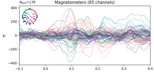
Generating an evoked response#
With the data preprocessed, it is now possible to see an auditory evoked response at the sensor level.
events = mne.find_events(raw, min_duration=0.1)
epochs = mne.Epochs(
    raw, events, tmin=-0.1, tmax=0.4, baseline=(-0.1, 0.0), verbose="error"
)
evoked = epochs.average()
evoked.plot()
180 events found
Event IDs: [3]
NOTE: pick_channels() is a legacy function. New code should use inst.pick(...).
References#
Total running time of the script: ( 0 minutes 19.110 seconds)
Estimated memory usage: 401 MB