mne_nirs.visualisation.plot_3d_montage

mne_nirs.visualisation.plot_3d_montage(info, view_map, *, src_det_names='auto', ch_names='numbered', subject='fsaverage', trans='fsaverage', surface='pial', subjects_dir=None, verbose=None)

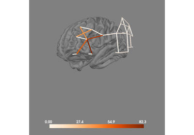
Plot a 3D sensor montage.

Parameters:

infoinstance of Info

Measurement info.

view_mapdict

Dict of view (key) to channel-pair-numbers (value) to use when plotting. Note that, because these get plotted as 1-based channel numbers, the values should be 1-based rather than 0-based. The keys are of the form:

'{side}-{view}'

For views like 'left-lat' or 'right-frontal' where the side matters.

'{view}'

For views like 'caudal' that are along the midline.

See mne.viz.Brain.show_view() for view options, and the Examples section below for usage examples.

src_det_namesNone | dict | str

Source and detector names to use. “auto” (default) will see if the channel locations correspond to standard 10-20 locations and will use those if they do (otherwise will act like None). None will use S1, S2, …, D1, D2, …, etc. Can also be an explicit dict mapping, for example:

src_det_names=dict(S1='Fz', D1='FCz', ...)

ch_namesstr | dict | None

If 'numbered' (default), use ['1', '2', ...] for the channel names, or None to use ['S1_D2', 'S2_D1', ...]. Can also be a dict to provide a mapping from the 'S1_D2'-style names (keys) to other names, e.g., defaultdict(lambda: '') will prevent showing the names altogether.

New in version 0.3.

subjectstr

The subject.

transstr | Transform

The subjects head<->MRI transform.

surfacestr

The FreeSurfer surface name (e.g., ‘pial’, ‘white’).

subjects_dirstr

The subjects directory.

verbosebool | str | int | None

Control verbosity of the logging output. If None, use the default verbosity level. See the logging documentation and mne.verbose() for details. Should only be passed as a keyword argument.

Returns:

figurematplotlib.figure.Figure

The matplotlib figimage.

Examples

For a Hitachi system with two sets of 12 source-detector arrangements, one on each side of the head, showing 1-12 on the left and 13-24 on the right can be accomplished using the following view_map:

>>> view_map = {
...     'left-lat': np.arange(1, 13),
...     'right-lat': np.arange(13, 25),
... }

NIRx typically involves more complicated arrangements. See the 3D tutorial for an advanced example that incorporates the 'caudal' view as well.

Examples using mne_nirs.visualisation.plot_3d_montage

Utilising Anatomical Information

Utilising Anatomical Information