mne.Evoked
- class mne.Evoked(fname, condition=None, proj=True, kind='average', allow_maxshield=False, verbose=None)[source]
Evoked data.
- Parameters
- fname
str Name of evoked/average FIF file to load. If None no data is loaded.
- condition
int, orstr Dataset ID number (int) or comment/name (str). Optional if there is only one data set in file.
- projbool, optional
Apply SSP projection vectors.
- kind
str Either ‘average’ or ‘standard_error’. The type of data to read. Only used if ‘condition’ is a str.
- allow_maxshieldbool |
str(defaultFalse) If True, allow loading of data that has been recorded with internal active compensation (MaxShield). Data recorded with MaxShield should generally not be loaded directly, but should first be processed using SSS/tSSS to remove the compensation signals that may also affect brain activity. Can also be “yes” to load without eliciting a warning.
- verbosebool,
str,int, orNone If not None, override default verbose level (see
mne.verbose()and Logging documentation for more). If used, it should be passed as a keyword-argument only.
- fname
Notes
Evoked objects can only contain the average of a single set of conditions.
- Attributes
- info
dict Measurement info.
ch_nameslistofstrChannel names.
- nave
int Number of averaged epochs.
kindstrThe data kind.
- comment
str Comment on dataset. Can be the condition.
dataarrayof shape (n_channels, n_times)The data matrix.
- first
int First time sample.
- last
int Last time sample.
tminfloatFirst time point.
tmaxfloatLast time point.
- times
array Time vector in seconds. Goes from
tmintotmax. Time interval between consecutive time samples is equal to the inverse of the sampling frequency.- baseline
None|tupleof length 2 This attribute reflects whether the data has been baseline-corrected (it will be a
tuplethen) or not (it will beNone).- verbosebool,
str,int, orNone If not None, override default verbose level (see
mne.verbose()and Logging documentation for more). If used, it should be passed as a keyword-argument only.
- info
Methods
__contains__(ch_type)Check channel type membership.
__hash__()Hash the object.
__neg__()Negate channel responses.
add_channels(add_list[, force_update_info])Append new channels to the instance.
add_proj(projs[, remove_existing, verbose])Add SSP projection vectors.
add_reference_channels(ref_channels)Add reference channels to data that consists of all zeros.
animate_topomap([ch_type, times, …])Make animation of evoked data as topomap timeseries.
anonymize([daysback, keep_his, verbose])Anonymize measurement information in place.
apply_baseline([baseline, verbose])Baseline correct evoked data.
apply_function(fun[, picks, dtype, n_jobs, …])Apply a function to a subset of channels.
apply_hilbert([picks, envelope, n_jobs, …])Compute analytic signal or envelope for a subset of channels.
apply_proj([verbose])Apply the signal space projection (SSP) operators to the data.
as_type([ch_type, mode])Compute virtual evoked using interpolated fields.
copy()Copy the instance of evoked.
crop([tmin, tmax, include_tmax, verbose])Crop data to a given time interval.
decimate(decim[, offset, verbose])Decimate the evoked data.
del_proj([idx])Remove SSP projection vector.
detrend([order, picks])Detrend data.
drop_channels(ch_names)Drop channel(s).
filter(l_freq, h_freq[, picks, …])Filter a subset of channels.
get_channel_types([picks, unique, only_data_chs])Get a list of channel type for each channel.
Get a DigMontage from instance.
get_peak([ch_type, tmin, tmax, mode, …])Get location and latency of peak amplitude.
interpolate_bads([reset_bads, mode, origin, …])Interpolate bad MEG and EEG channels.
pick(picks[, exclude])Pick a subset of channels.
pick_channels(ch_names[, ordered])Pick some channels.
pick_types([meg, eeg, stim, eog, ecg, emg, …])Pick some channels by type and names.
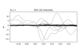
plot([picks, exclude, unit, show, ylim, …])Plot evoked data using butterfly plots.
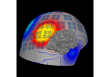
plot_field(surf_maps[, time, time_label, …])Plot MEG/EEG fields on head surface and helmet in 3D.
plot_image([picks, exclude, unit, show, …])Plot evoked data as images.
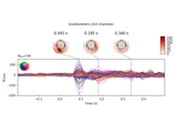
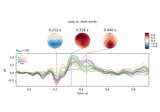
plot_joint([times, title, picks, exclude, …])Plot evoked data as butterfly plot and add topomaps for time points.
plot_projs_topomap([ch_type, cmap, sensors, …])Plot SSP vector.
plot_sensors([kind, ch_type, title, …])Plot sensor positions.
plot_topo([layout, layout_scale, color, …])Plot 2D topography of evoked responses.
plot_topomap([times, ch_type, vmin, vmax, …])Plot topographic maps of specific time points of evoked data.
plot_white(noise_cov[, show, rank, …])Plot whitened evoked response.
rename_channels(mapping[, allow_duplicates, …])Rename channels.
reorder_channels(ch_names)Reorder channels.
resample(sfreq[, npad, window, n_jobs, pad, …])Resample data.
save(fname)Save dataset to file.
savgol_filter(h_freq[, verbose])Filter the data using Savitzky-Golay polynomial method.
set_channel_types(mapping[, verbose])Define the sensor type of channels.
set_eeg_reference([ref_channels, …])Specify which reference to use for EEG data.
set_meas_date(meas_date)Set the measurement start date.
set_montage(montage[, match_case, …])Set EEG sensor configuration and head digitization.
shift_time(tshift[, relative])Shift time scale in epoched or evoked data.
time_as_index(times[, use_rounding])Convert time to indices.
to_data_frame([picks, index, scalings, …])Export data in tabular structure as a pandas DataFrame.
- __contains__(ch_type)[source]
Check channel type membership.
- Parameters
- ch_type
str Channel type to check for. Can be e.g. ‘meg’, ‘eeg’, ‘stim’, etc.
- ch_type
- Returns
- inbool
Whether or not the instance contains the given channel type.
Examples
Channel type membership can be tested as:
>>> 'meg' in inst
True
>>> 'seeg' in inst
False
- __neg__()[source]
Negate channel responses.
- Returns
- evoked_neginstance of
Evoked The Evoked instance with channel data negated and ‘-‘ prepended to the comment.
- evoked_neginstance of
- add_channels(add_list, force_update_info=False)[source]
Append new channels to the instance.
- Parameters
- add_list
list A list of objects to append to self. Must contain all the same type as the current object.
- force_update_infobool
If True, force the info for objects to be appended to match the values in
self. This should generally only be used when adding stim channels for which important metadata won’t be overwritten.New in version 0.12.
- add_list
- Returns
See also
Notes
If
selfis a Raw instance that has been preloaded into anumpy.memmapinstance, the memmap will be resized.
- add_proj(projs, remove_existing=False, verbose=None)[source]
Add SSP projection vectors.
- Parameters
- projs
list List with projection vectors.
- remove_existingbool
Remove the projection vectors currently in the file.
- verbosebool,
str,int, orNone If not None, override default verbose level (see
mne.verbose()and Logging documentation for more). If used, it should be passed as a keyword-argument only. Defaults to self.verbose.
- projs
- Returns
Examples using
add_proj:
- add_reference_channels(ref_channels)[source]
Add reference channels to data that consists of all zeros.
Adds reference channels to data that were not included during recording. This is useful when you need to re-reference your data to different channels. These added channels will consist of all zeros.
- Parameters
- Returns
- animate_topomap(ch_type=None, times=None, frame_rate=None, butterfly=False, blit=True, show=True, time_unit='s', sphere=None, *, extrapolate='auto', verbose=None)[source]
Make animation of evoked data as topomap timeseries.
The animation can be paused/resumed with left mouse button. Left and right arrow keys can be used to move backward or forward in time.
- Parameters
- ch_type
str|None Channel type to plot. Accepted data types: ‘mag’, ‘grad’, ‘eeg’, ‘hbo’, ‘hbr’, ‘fnirs_cw_amplitude’, ‘fnirs_fd_ac_amplitude’, ‘fnirs_fd_phase’, and ‘fnirs_od’. If None, first available channel type from the above list is used. Defaults to None.
- times
arrayoffloat|None The time points to plot. If None, 10 evenly spaced samples are calculated over the evoked time series. Defaults to None.
- frame_rate
int|None Frame rate for the animation in Hz. If None, frame rate = sfreq / 10. Defaults to None.
- butterflybool
Whether to plot the data as butterfly plot under the topomap. Defaults to False.
- blitbool
Whether to use blit to optimize drawing. In general, it is recommended to use blit in combination with
show=True. If you intend to save the animation it is better to disable blit. Defaults to True.- showbool
Whether to show the animation. Defaults to True.
- time_unit
str The units for the time axis, can be “ms” (default in 0.16) or “s” (will become the default in 0.17).
New in version 0.16.
- sphere
float| array_like |str|None The sphere parameters to use for the cartoon head. Can be array-like of shape (4,) to give the X/Y/Z origin and radius in meters, or a single float to give the radius (origin assumed 0, 0, 0). Can also be a spherical ConductorModel, which will use the origin and radius. Can be “auto” to use a digitization-based fit. Can also be None (default) to use ‘auto’ when enough extra digitization points are available, and 0.095 otherwise. Currently the head radius does not affect plotting.
New in version 0.20.
- extrapolate
str Options:
'box'Extrapolate to four points placed to form a square encompassing all data points, where each side of the square is three times the range of the data in the respective dimension.
'local'(default)Extrapolate only to nearby points (approximately to points closer than median inter-electrode distance). This will also set the mask to be polygonal based on the convex hull of the sensors.
'head'Extrapolate out to the edges of the clipping circle. This will be on the head circle when the sensors are contained within the head circle, but it can extend beyond the head when sensors are plotted outside the head circle.
Changed in version 0.21:
The default was changed to
'local''local'was changed to use a convex hull mask'head'was changed to extrapolate out to the clipping circle.
New in version 0.22.
- verbosebool,
str,int, orNone If not None, override default verbose level (see
mne.verbose()and Logging documentation for more). If used, it should be passed as a keyword-argument only. Defaults to self.verbose.
- ch_type
- Returns
- figinstance of
matplotlib.figure.Figure The figure.
- animinstance of
matplotlib.animation.FuncAnimation Animation of the topomap.
- figinstance of
Notes
New in version 0.12.0.
Examples using
animate_topomap:
- anonymize(daysback=None, keep_his=False, verbose=None)[source]
Anonymize measurement information in place.
- Parameters
- daysback
int|None Number of days to subtract from all dates. If
None(default), the acquisition date,info['meas_date'], will be set toJanuary 1ˢᵗ, 2000. This parameter is ignored ifinfo['meas_date']isNone(i.e., no acquisition date has been set).- keep_hisbool
If
True,his_idofsubject_infowill not be overwritten. Defaults toFalse.Warning
This could mean that
infois not fully anonymized. Use with caution.- verbosebool,
str,int, orNone If not None, override default verbose level (see
mne.verbose()and Logging documentation for more). If used, it should be passed as a keyword-argument only.
- daysback
- Returns
Notes
Removes potentially identifying information if it exists in
info. Specifically for each of the following we use:- meas_date, file_id, meas_id
A default value, or as specified by
daysback.
- subject_info
Default values, except for ‘birthday’ which is adjusted to maintain the subject age.
- experimenter, proj_name, description
Default strings.
- utc_offset
None.
- proj_id
Zeros.
- proc_history
Dates use the
meas_datelogic, and experimenter a default string.
- helium_info, device_info
Dates use the
meas_datelogic, meta info uses defaults.
If
info['meas_date']isNone, it will remainNoneduring processing the above fields.Operates in place.
New in version 0.13.0.
- apply_baseline(baseline=(None, 0), *, verbose=None)[source]
Baseline correct evoked data.
- Parameters
- baseline
None|tupleof length 2 The time interval to consider as “baseline” when applying baseline correction. If
None, do not apply baseline correction. If a tuple(a, b), the interval is betweenaandb(in seconds), including the endpoints. IfaisNone, the beginning of the data is used; and ifbisNone, it is set to the end of the interval. If(None, None), the entire time interval is used.Note
The baseline
(a, b)includes both endpoints, i.e. all timepointstsuch thata <= t <= b.Correction is applied to each channel individually in the following way:
Calculate the mean signal of the baseline period.
Subtract this mean from the entire
Evoked.
Defaults to
(None, 0), i.e. beginning of the the data until time point zero.- verbosebool,
str,int, orNone If not None, override default verbose level (see
mne.verbose()and Logging documentation for more). If used, it should be passed as a keyword-argument only. Defaults to self.verbose.
- baseline
- Returns
- evokedinstance of
Evoked The baseline-corrected Evoked object.
- evokedinstance of
Notes
Baseline correction can be done multiple times.
New in version 0.13.0.
Examples using
apply_baseline:
- apply_function(fun, picks=None, dtype=None, n_jobs=1, verbose=None, **kwargs)[source]
Apply a function to a subset of channels.
The function
funis applied to the channels defined inpicks. The evoked object’s data is modified in-place. If the function returns a different data type (e.g.numpy.complex128) it must be specified using thedtypeparameter, which causes the data type of all the data to change (even if the function is only applied to channels inpicks).Note
If
n_jobs> 1, more memory is required aslen(picks) * n_timesadditional time points need to be temporarily stored in memory.Note
If the data type changes (
dtype != None), more memory is required since the original and the converted data needs to be stored in memory.- Parameters
- fun
callable() A function to be applied to the channels. The first argument of fun has to be a timeseries (
numpy.ndarray). The function must operate on an array of shape(n_times,)because it will apply channel-wise. The function must return anndarrayshaped like its input.- picks
str|list|slice|None Channels to include. Slices and lists of integers will be interpreted as channel indices. In lists, channel type strings (e.g.,
['meg', 'eeg']) will pick channels of those types, channel name strings (e.g.,['MEG0111', 'MEG2623']will pick the given channels. Can also be the string values “all” to pick all channels, or “data” to pick data channels. None (default) will pick all data channels (excluding reference MEG channels). Note that channels ininfo['bads']will be included if their names or indices are explicitly provided.- dtype
numpy.dtype Data type to use after applying the function. If None (default) the data type is not modified.
- n_jobs
int The number of jobs to run in parallel (default 1). Requires the joblib package.
- verbosebool,
str,int, orNone If not None, override default verbose level (see
mne.verbose()and Logging documentation for more). If used, it should be passed as a keyword-argument only. Defaults to self.verbose.- **kwargs
dict Additional keyword arguments to pass to
fun.
- fun
- Returns
- selfinstance of
Evoked The evoked object with transformed data.
- selfinstance of
- apply_hilbert(picks=None, envelope=False, n_jobs=1, n_fft='auto', verbose=None)[source]
Compute analytic signal or envelope for a subset of channels.
- Parameters
- picks
str|list|slice|None Channels to include. Slices and lists of integers will be interpreted as channel indices. In lists, channel type strings (e.g.,
['meg', 'eeg']) will pick channels of those types, channel name strings (e.g.,['MEG0111', 'MEG2623']will pick the given channels. Can also be the string values “all” to pick all channels, or “data” to pick data channels. None (default) will pick all data channels (excluding reference MEG channels). Note that channels ininfo['bads']will be included if their names or indices are explicitly provided.- envelopebool
Compute the envelope signal of each channel. Default False. See Notes.
- n_jobs
int The number of jobs to run in parallel (default 1). Requires the joblib package.
- n_fft
int|None|str Points to use in the FFT for Hilbert transformation. The signal will be padded with zeros before computing Hilbert, then cut back to original length. If None, n == self.n_times. If ‘auto’, the next highest fast FFT length will be use.
- verbosebool,
str,int, orNone If not None, override default verbose level (see
mne.verbose()and Logging documentation for more). If used, it should be passed as a keyword-argument only. Defaults to self.verbose.
- picks
- Returns
Notes
Parameters
If
envelope=False, the analytic signal for the channels defined inpicksis computed and the data of the Raw object is converted to a complex representation (the analytic signal is complex valued).If
envelope=True, the absolute value of the analytic signal for the channels defined inpicksis computed, resulting in the envelope signal.If envelope=False, more memory is required since the original raw data as well as the analytic signal have temporarily to be stored in memory. If n_jobs > 1, more memory is required as
len(picks) * n_timesadditional time points need to be temporaily stored in memory.Also note that the
n_fftparameter will allow you to pad the signal with zeros before performing the Hilbert transform. This padding is cut off, but it may result in a slightly different result (particularly around the edges). Use at your own risk.Analytic signal
The analytic signal “x_a(t)” of “x(t)” is:
x_a = F^{-1}(F(x) 2U) = x + i y
where “F” is the Fourier transform, “U” the unit step function, and “y” the Hilbert transform of “x”. One usage of the analytic signal is the computation of the envelope signal, which is given by “e(t) = abs(x_a(t))”. Due to the linearity of Hilbert transform and the MNE inverse solution, the enevlope in source space can be obtained by computing the analytic signal in sensor space, applying the MNE inverse, and computing the envelope in source space.
- apply_proj(verbose=None)[source]
Apply the signal space projection (SSP) operators to the data.
- Parameters
- verbosebool,
str,int, orNone If not None, override default verbose level (see
mne.verbose()and Logging documentation for more). If used, it should be passed as a keyword-argument only. Defaults to self.verbose.
- verbosebool,
- Returns
Notes
Once the projectors have been applied, they can no longer be removed. It is usually not recommended to apply the projectors at too early stages, as they are applied automatically later on (e.g. when computing inverse solutions). Hint: using the copy method individual projection vectors can be tested without affecting the original data. With evoked data, consider the following example:
projs_a = mne.read_proj('proj_a.fif')
projs_b = mne.read_proj('proj_b.fif')
# add the first, copy, apply and see ...
evoked.add_proj(a).copy().apply_proj().plot()
# add the second, copy, apply and see ...
evoked.add_proj(b).copy().apply_proj().plot()
# drop the first and see again
evoked.copy().del_proj(0).apply_proj().plot()
evoked.apply_proj()  # finally keep both
Examples using
apply_proj:
- as_type(ch_type='grad', mode='fast')[source]
Compute virtual evoked using interpolated fields.
Warning
Using virtual evoked to compute inverse can yield unexpected results. The virtual channels have
'_v'appended at the end of the names to emphasize that the data contained in them are interpolated.- Parameters
- Returns
- evokedinstance of
mne.Evoked The transformed evoked object containing only virtual channels.
- evokedinstance of
Notes
This method returns a copy and does not modify the data it operates on. It also returns an EvokedArray instance.
New in version 0.9.0.
Examples using
as_type:
- property ch_names
Channel names.
- property compensation_grade
The current gradient compensation grade.
- copy()[source]
Copy the instance of evoked.
- Returns
- evokedinstance of
Evoked A copy of the object.
- evokedinstance of
Examples using
copy:
- crop(tmin=None, tmax=None, include_tmax=True, verbose=None)[source]
Crop data to a given time interval.
- Parameters
- tmin
float|None Start time of selection in seconds.
- tmax
float|None End time of selection in seconds.
- include_tmaxbool
If True (default), include tmax. If False, exclude tmax (similar to how Python indexing typically works).
New in version 0.19.
- verbosebool,
str,int, orNone If not None, override default verbose level (see
mne.verbose()and Logging documentation for more). If used, it should be passed as a keyword-argument only. Defaults to self.verbose.
- tmin
- Returns
- evokedinstance of
Evoked The cropped Evoked object, modified in-place.
- evokedinstance of
Notes
Unlike Python slices, MNE time intervals by default include both their end points;
crop(tmin, tmax)returns the intervaltmin <= t <= tmax. Passinclude_tmax=Falseto specify the half-open intervaltmin <= t < tmaxinstead.Examples using
crop:
- property data
The data matrix.
- decimate(decim, offset=0, verbose=None)[source]
Decimate the evoked data.
- Parameters
- decim
int Factor by which to subsample the data.
Warning
Low-pass filtering is not performed, this simply selects every Nth sample (where N is the value passed to
decim), i.e., it compresses the signal (see Notes). If the data are not properly filtered, aliasing artifacts may occur.- offset
int Apply an offset to where the decimation starts relative to the sample corresponding to t=0. The offset is in samples at the current sampling rate.
New in version 0.12.
- verbosebool,
str,int, orNone If not None, override default verbose level (see
mne.verbose()and Logging documentation for more). If used, it should be passed as a keyword-argument only. Defaults to self.verbose.
- decim
- Returns
- evokedinstance of
Evoked The decimated Evoked object.
- evokedinstance of
Notes
For historical reasons,
decim/ “decimation” refers to simply subselecting samples from a given signal. This contrasts with the broader signal processing literature, where decimation is defined as (quoting 1, p. 172; which cites 2):“… a general system for downsampling by a factor of M is the one shown in Figure 4.23. Such a system is called a decimator, and downsampling by lowpass filtering followed by compression [i.e, subselecting samples] has been termed decimation (Crochiere and Rabiner, 1983).”
Hence “decimation” in MNE is what is considered “compression” in the signal processing community.
Decimation can be done multiple times. For example,
inst.decimate(2).decimate(2)will be the same asinst.decimate(4).New in version 0.13.0.
Examples using
decimate:
- del_proj(idx='all')[source]
Remove SSP projection vector.
Note
The projection vector can only be removed if it is inactive (has not been applied to the data).
- Parameters
- Returns
Examples using
del_proj:
- detrend(order=1, picks=None)[source]
Detrend data.
This function operates in-place.
- Parameters
- order
int Either 0 or 1, the order of the detrending. 0 is a constant (DC) detrend, 1 is a linear detrend.
- picks
str|list|slice|None Channels to include. Slices and lists of integers will be interpreted as channel indices. In lists, channel type strings (e.g.,
['meg', 'eeg']) will pick channels of those types, channel name strings (e.g.,['MEG0111', 'MEG2623']will pick the given channels. Can also be the string values “all” to pick all channels, or “data” to pick data channels. None (default) will pick good data channels. Note that channels ininfo['bads']will be included if their names or indices are explicitly provided.
- order
- Returns
- evokedinstance of
Evoked The detrended evoked object.
- evokedinstance of
- drop_channels(ch_names)[source]
Drop channel(s).
- Parameters
- Returns
See also
Notes
New in version 0.9.0.
Examples using
drop_channels:
- filter(l_freq, h_freq, picks=None, filter_length='auto', l_trans_bandwidth='auto', h_trans_bandwidth='auto', n_jobs=1, method='fir', iir_params=None, phase='zero', fir_window='hamming', fir_design='firwin', skip_by_annotation=('edge', 'bad_acq_skip'), pad='edge', verbose=None)[source]
Filter a subset of channels.
- Parameters
- l_freq
float|None For FIR filters, the lower pass-band edge; for IIR filters, the lower cutoff frequency. If None the data are only low-passed.
- h_freq
float|None For FIR filters, the upper pass-band edge; for IIR filters, the upper cutoff frequency. If None the data are only high-passed.
- picks
str|list|slice|None Channels to include. Slices and lists of integers will be interpreted as channel indices. In lists, channel type strings (e.g.,
['meg', 'eeg']) will pick channels of those types, channel name strings (e.g.,['MEG0111', 'MEG2623']will pick the given channels. Can also be the string values “all” to pick all channels, or “data” to pick data channels. None (default) will pick all data channels. Note that channels ininfo['bads']will be included if their names or indices are explicitly provided.- filter_length
str|int Length of the FIR filter to use (if applicable):
‘auto’ (default): The filter length is chosen based on the size of the transition regions (6.6 times the reciprocal of the shortest transition band for fir_window=’hamming’ and fir_design=”firwin2”, and half that for “firwin”).
str: A human-readable time in units of “s” or “ms” (e.g., “10s” or “5500ms”) will be converted to that number of samples if
phase="zero", or the shortest power-of-two length at least that duration forphase="zero-double".int: Specified length in samples. For fir_design=”firwin”, this should not be used.
- l_trans_bandwidth
float|str Width of the transition band at the low cut-off frequency in Hz (high pass or cutoff 1 in bandpass). Can be “auto” (default) to use a multiple of
l_freq:min(max(l_freq * 0.25, 2), l_freq)
Only used for
method='fir'.- h_trans_bandwidth
float|str Width of the transition band at the high cut-off frequency in Hz (low pass or cutoff 2 in bandpass). Can be “auto” (default in 0.14) to use a multiple of
h_freq:min(max(h_freq * 0.25, 2.), info['sfreq'] / 2. - h_freq)
Only used for
method='fir'.- n_jobs
int|str Number of jobs to run in parallel. Can be ‘cuda’ if
cupyis installed properly and method=’fir’.- method
str ‘fir’ will use overlap-add FIR filtering, ‘iir’ will use IIR forward-backward filtering (via filtfilt).
- iir_params
dict|None Dictionary of parameters to use for IIR filtering. If iir_params is None and method=”iir”, 4th order Butterworth will be used. For more information, see
mne.filter.construct_iir_filter().- phase
str Phase of the filter, only used if
method='fir'. Symmetric linear-phase FIR filters are constructed, and ifphase='zero'(default), the delay of this filter is compensated for, making it non-causal. Ifphase=='zero-double', then this filter is applied twice, once forward, and once backward (also making it non-causal). If ‘minimum’, then a minimum-phase filter will be constricted and applied, which is causal but has weaker stop-band suppression.New in version 0.13.
- fir_window
str The window to use in FIR design, can be “hamming” (default), “hann” (default in 0.13), or “blackman”.
New in version 0.15.
- fir_design
str Can be “firwin” (default) to use
scipy.signal.firwin(), or “firwin2” to usescipy.signal.firwin2(). “firwin” uses a time-domain design technique that generally gives improved attenuation using fewer samples than “firwin2”.New in version 0.15.
- skip_by_annotation
str|listofstr If a string (or list of str), any annotation segment that begins with the given string will not be included in filtering, and segments on either side of the given excluded annotated segment will be filtered separately (i.e., as independent signals). The default (
('edge', 'bad_acq_skip')will separately filter any segments that were concatenated bymne.concatenate_raws()ormne.io.Raw.append(), or separated during acquisition. To disable, provide an empty list. Only used ifinstis raw.New in version 0.16..
- pad
str The type of padding to use. Supports all
numpy.pad()modeoptions. Can also be “reflect_limited”, which pads with a reflected version of each vector mirrored on the first and last values of the vector, followed by zeros. Only used formethod='fir'.- verbosebool,
str,int, orNone If not None, override default verbose level (see
mne.verbose()and Logging documentation for more). If used, it should be passed as a keyword-argument only. Defaults to self.verbose.
- l_freq
- Returns
See also
Notes
Applies a zero-phase low-pass, high-pass, band-pass, or band-stop filter to the channels selected by
picks. The data are modified inplace.The object has to have the data loaded e.g. with
preload=Trueorself.load_data().l_freqandh_freqare the frequencies below which and above which, respectively, to filter out of the data. Thus the uses are:l_freq < h_freq: band-pass filterl_freq > h_freq: band-stop filterl_freq is not None and h_freq is None: high-pass filterl_freq is None and h_freq is not None: low-pass filter
self.info['lowpass']andself.info['highpass']are only updated with picks=None.Note
If n_jobs > 1, more memory is required as
len(picks) * n_timesadditional time points need to be temporaily stored in memory.For more information, see the tutorials Background information on filtering and Filtering and resampling data and
mne.filter.create_filter().New in version 0.15.
Examples using
filter:
- get_channel_types(picks=None, unique=False, only_data_chs=False)[source]
Get a list of channel type for each channel.
- Parameters
- picks
str|list|slice|None Channels to include. Slices and lists of integers will be interpreted as channel indices. In lists, channel type strings (e.g.,
['meg', 'eeg']) will pick channels of those types, channel name strings (e.g.,['MEG0111', 'MEG2623']will pick the given channels. Can also be the string values “all” to pick all channels, or “data” to pick data channels. None (default) will pick all channels. Note that channels ininfo['bads']will be included if their names or indices are explicitly provided.- uniquebool
Whether to return only unique channel types. Default is
False.- only_data_chsbool
Whether to ignore non-data channels. Default is
False.
- picks
- Returns
- channel_types
list The channel types.
- channel_types
- get_montage()[source]
Get a DigMontage from instance.
- Returns
- montage
None|str|DigMontage A montage containing channel positions. If str or DigMontage is specified, the channel info will be updated with the channel positions. Default is None. For valid
strvalues see documentation ofmne.channels.make_standard_montage(). See also the documentation ofmne.channels.DigMontagefor more information.
- montage
- get_peak(ch_type=None, tmin=None, tmax=None, mode='abs', time_as_index=False, merge_grads=False, return_amplitude=False)[source]
Get location and latency of peak amplitude.
- Parameters
- ch_type
str|None The channel type to use. Defaults to None. If more than one sensor Type is present in the data the channel type has to be explicitly set.
- tmin
float|None The minimum point in time to be considered for peak getting. If None (default), the beginning of the data is used.
- tmax
float|None The maximum point in time to be considered for peak getting. If None (default), the end of the data is used.
- mode{‘pos’, ‘neg’, ‘abs’}
How to deal with the sign of the data. If ‘pos’ only positive values will be considered. If ‘neg’ only negative values will be considered. If ‘abs’ absolute values will be considered. Defaults to ‘abs’.
- time_as_indexbool
Whether to return the time index instead of the latency in seconds.
- merge_gradsbool
If True, compute peak from merged gradiometer data.
- return_amplitudebool
If True, return also the amplitude at the maximum response.
New in version 0.16.
- ch_type
- Returns
Examples using
get_peak:
- interpolate_bads(reset_bads=True, mode='accurate', origin='auto', method=None, exclude=(), verbose=None)[source]
Interpolate bad MEG and EEG channels.
Operates in place.
- Parameters
- reset_badsbool
If True, remove the bads from info.
- mode
str Either
'accurate'or'fast', determines the quality of the Legendre polynomial expansion used for interpolation of channels using the minimum-norm method.- originarray_like, shape (3,) |
str Origin of the sphere in the head coordinate frame and in meters. Can be
'auto'(default), which means a head-digitization-based origin fit.New in version 0.17.
- method
dict Method to use for each channel type. Currently only the key “eeg” has multiple options:
"spline"(default)Use spherical spline interpolation.
"MNE"Use minimum-norm projection to a sphere and back. This is the method used for MEG channels.
The value for “meg” is “MNE”, and the value for “fnirs” is “nearest”. The default (None) is thus an alias for:
method=dict(meg="MNE", eeg="spline", fnirs="nearest")
New in version 0.21.
- exclude
list|tuple The channels to exclude from interpolation. If excluded a bad channel will stay in bads.
- verbosebool,
str,int, orNone If not None, override default verbose level (see
mne.verbose()and Logging documentation for more). If used, it should be passed as a keyword-argument only. Defaults to self.verbose.
- Returns
Notes
New in version 0.9.0.
- property kind
The data kind.
- pick(picks, exclude=())[source]
Pick a subset of channels.
- Parameters
- picks
str|list|slice|None Channels to include. Slices and lists of integers will be interpreted as channel indices. In lists, channel type strings (e.g.,
['meg', 'eeg']) will pick channels of those types, channel name strings (e.g.,['MEG0111', 'MEG2623']will pick the given channels. Can also be the string values “all” to pick all channels, or “data” to pick data channels. None (default) will pick all channels. Note that channels ininfo['bads']will be included if their names or indices are explicitly provided.- exclude
list|str Set of channels to exclude, only used when picking based on types (e.g., exclude=”bads” when picks=”meg”).
- picks
- Returns
Examples using
pick:
- pick_channels(ch_names, ordered=False)[source]
Pick some channels.
- Parameters
- Returns
See also
Notes
The channel names given are assumed to be a set, i.e. the order does not matter. The original order of the channels is preserved. You can use
reorder_channelsto set channel order if necessary.New in version 0.9.0.
Examples using
pick_channels:
- pick_types(meg=False, eeg=False, stim=False, eog=False, ecg=False, emg=False, ref_meg='auto', misc=False, resp=False, chpi=False, exci=False, ias=False, syst=False, seeg=False, dipole=False, gof=False, bio=False, ecog=False, fnirs=False, csd=False, dbs=False, include=(), exclude='bads', selection=None, verbose=None)[source]
Pick some channels by type and names.
- Parameters
- megbool |
str If True include MEG channels. If string it can be ‘mag’, ‘grad’, ‘planar1’ or ‘planar2’ to select only magnetometers, all gradiometers, or a specific type of gradiometer.
- eegbool
If True include EEG channels.
- stimbool
If True include stimulus channels.
- eogbool
If True include EOG channels.
- ecgbool
If True include ECG channels.
- emgbool
If True include EMG channels.
- ref_megbool |
str If True include CTF / 4D reference channels. If ‘auto’, reference channels are included if compensations are present and
megis not False. Can also be the string options for themegparameter.- miscbool
If True include miscellaneous analog channels.
- respbool
If
Trueinclude respiratory channels.- chpibool
If True include continuous HPI coil channels.
- excibool
Flux excitation channel used to be a stimulus channel.
- iasbool
Internal Active Shielding data (maybe on Triux only).
- systbool
System status channel information (on Triux systems only).
- seegbool
Stereotactic EEG channels.
- dipolebool
Dipole time course channels.
- gofbool
Dipole goodness of fit channels.
- biobool
Bio channels.
- ecogbool
Electrocorticography channels.
- fnirsbool |
str Functional near-infrared spectroscopy channels. If True include all fNIRS channels. If False (default) include none. If string it can be ‘hbo’ (to include channels measuring oxyhemoglobin) or ‘hbr’ (to include channels measuring deoxyhemoglobin).
- csdbool
EEG-CSD channels.
- dbsbool
Deep brain stimulation channels.
- include
listofstr List of additional channels to include. If empty do not include any.
- exclude
listofstr|str List of channels to exclude. If ‘bads’ (default), exclude channels in
info['bads'].- selection
listofstr Restrict sensor channels (MEG, EEG) to this list of channel names.
- verbosebool,
str,int, orNone If not None, override default verbose level (see
mne.verbose()and Logging documentation for more). If used, it should be passed as a keyword-argument only. Defaults to self.verbose.
- megbool |
- Returns
See also
Notes
New in version 0.9.0.
Examples using
pick_types:
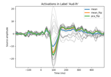
- plot(picks=None, exclude='bads', unit=True, show=True, ylim=None, xlim='tight', proj=False, hline=None, units=None, scalings=None, titles=None, axes=None, gfp=False, window_title=None, spatial_colors=False, zorder='unsorted', selectable=True, noise_cov=None, time_unit='s', sphere=None, verbose=None)[source]
Plot evoked data using butterfly plots.
Left click to a line shows the channel name. Selecting an area by clicking and holding left mouse button plots a topographic map of the painted area.
Note
If bad channels are not excluded they are shown in red.
- Parameters
- picks
str|list|slice|None Channels to include. Slices and lists of integers will be interpreted as channel indices. In lists, channel type strings (e.g.,
['meg', 'eeg']) will pick channels of those types, channel name strings (e.g.,['MEG0111', 'MEG2623']will pick the given channels. Can also be the string values “all” to pick all channels, or “data” to pick data channels. None (default) will pick all channels. Note that channels ininfo['bads']will be included if their names or indices are explicitly provided.- exclude
listofstr| ‘bads’ Channels names to exclude from being shown. If ‘bads’, the bad channels are excluded.
- unitbool
Scale plot with channel (SI) unit.
- showbool
Show figure if True.
- ylim
dict|None Y limits for plots (after scaling has been applied). e.g. ylim = dict(eeg=[-20, 20]) Valid keys are eeg, mag, grad, misc. If None, the ylim parameter for each channel equals the pyplot default.
- xlim‘tight’ |
tuple|None X limits for plots.
- projbool | ‘interactive’ | ‘reconstruct’
If true SSP projections are applied before display. If ‘interactive’, a check box for reversible selection of SSP projection vectors will be shown. If ‘reconstruct’, projection vectors will be applied and then M/EEG data will be reconstructed via field mapping to reduce the signal bias caused by projection.
Changed in version 0.21: Support for ‘reconstruct’ was added.
- hline
listoffloat|None The values at which to show an horizontal line.
- units
dict|None The units of the channel types used for axes labels. If None, defaults to
dict(eeg='µV', grad='fT/cm', mag='fT').- scalings
dict|None The scalings of the channel types to be applied for plotting. If None, defaults to
dict(eeg=1e6, grad=1e13, mag=1e15).- titles
dict|None The titles associated with the channels. If None, defaults to
dict(eeg='EEG', grad='Gradiometers', mag='Magnetometers').- axesinstance of
Axes|list|None The axes to plot to. If list, the list must be a list of Axes of the same length as the number of channel types. If instance of Axes, there must be only one channel type plotted.
- gfpbool | ‘only’
Plot the global field power (GFP) or the root mean square (RMS) of the data. For MEG data, this will plot the RMS. For EEG, it plots GFP, i.e. the standard deviation of the signal across channels. The GFP is equivalent to the RMS of an average-referenced signal.
TruePlot GFP or RMS (for EEG and MEG, respectively) and traces for all channels.
'only'Plot GFP or RMS (for EEG and MEG, respectively), and omit the traces for individual channels.
The color of the GFP/RMS trace will be green if
spatial_colors=False, and black otherwise.Changed in version 0.23: Plot GFP for EEG instead of RMS. Label RMS traces correctly as such.
- window_title
str|None The title to put at the top of the figure.
- spatial_colorsbool
If True, the lines are color coded by mapping physical sensor coordinates into color values. Spatially similar channels will have similar colors. Bad channels will be dotted. If False, the good channels are plotted black and bad channels red. Defaults to False.
- zorder
str|callable() Which channels to put in the front or back. Only matters if
spatial_colorsis used. If str, must bestdorunsorted(defaults tounsorted). Ifstd, data with the lowest standard deviation (weakest effects) will be put in front so that they are not obscured by those with stronger effects. Ifunsorted, channels are z-sorted as in the evoked instance. If callable, must take one argument: a numpy array of the same dimensionality as the evoked raw data; and return a list of unique integers corresponding to the number of channels.New in version 0.13.0.
- selectablebool
Whether to use interactive features. If True (default), it is possible to paint an area to draw topomaps. When False, the interactive features are disabled. Disabling interactive features reduces memory consumption and is useful when using
axesparameter to draw multiaxes figures.New in version 0.13.0.
- noise_covinstance of
Covariance|str|None Noise covariance used to whiten the data while plotting. Whitened data channel names are shown in italic. Can be a string to load a covariance from disk. See also
mne.Evoked.plot_white()for additional inspection of noise covariance properties when whitening evoked data. For data processed with SSS, the effective dependence between magnetometers and gradiometers may introduce differences in scaling, consider usingmne.Evoked.plot_white().New in version 0.16.0.
- time_unit
str The units for the time axis, can be “ms” or “s” (default).
New in version 0.16.
- sphere
float| array_like |str|None The sphere parameters to use for the cartoon head. Can be array-like of shape (4,) to give the X/Y/Z origin and radius in meters, or a single float to give the radius (origin assumed 0, 0, 0). Can also be a spherical ConductorModel, which will use the origin and radius. Can be “auto” to use a digitization-based fit. Can also be None (default) to use ‘auto’ when enough extra digitization points are available, and 0.095 otherwise. Currently the head radius does not affect plotting.
New in version 0.20.
- verbosebool,
str,int, orNone If not None, override default verbose level (see
mne.verbose()and Logging documentation for more). If used, it should be passed as a keyword-argument only.
- picks
- Returns
- figinstance of
matplotlib.figure.Figure Figure containing the butterfly plots.
- figinstance of
See also
Examples using
plot:
- plot_field(surf_maps, time=None, time_label='t = %0.0f ms', n_jobs=1, fig=None, vmax=None, n_contours=21, verbose=None)[source]
Plot MEG/EEG fields on head surface and helmet in 3D.
- Parameters
- surf_maps
list The surface mapping information obtained with make_field_map.
- time
float|None The time point at which the field map shall be displayed. If None, the average peak latency (across sensor types) is used.
- time_label
str|None How to print info about the time instant visualized.
- n_jobs
int The number of jobs to run in parallel (default 1). Requires the joblib package.
- figinstance of
mayavi.core.api.Scene|None If None (default), a new figure will be created, otherwise it will plot into the given figure.
New in version 0.20.
- vmax
float|None Maximum intensity. Can be None to use the max(abs(data)).
New in version 0.21.
- n_contours
int The number of contours.
New in version 0.21.
- verbosebool,
str,int, orNone If not None, override default verbose level (see
mne.verbose()and Logging documentation for more). If used, it should be passed as a keyword-argument only.
- surf_maps
- Returns
- figinstance of
mayavi.mlab.Figure The mayavi figure.
- figinstance of
Examples using
plot_field:
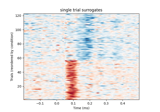
- plot_image(picks=None, exclude='bads', unit=True, show=True, clim=None, xlim='tight', proj=False, units=None, scalings=None, titles=None, axes=None, cmap='RdBu_r', colorbar=True, mask=None, mask_style=None, mask_cmap='Greys', mask_alpha=0.25, time_unit='s', show_names=None, group_by=None, sphere=None)[source]
Plot evoked data as images.
- Parameters
- picks
str|list|slice|None Channels to include. Slices and lists of integers will be interpreted as channel indices. In lists, channel type strings (e.g.,
['meg', 'eeg']) will pick channels of those types, channel name strings (e.g.,['MEG0111', 'MEG2623']will pick the given channels. Can also be the string values “all” to pick all channels, or “data” to pick data channels. None (default) will pick all channels. Note that channels ininfo['bads']will be included if their names or indices are explicitly provided. This parameter can also be used to set the order the channels are shown in, as the channel image is sorted by the order of picks.- exclude
listofstr| ‘bads’ Channels names to exclude from being shown. If ‘bads’, the bad channels are excluded.
- unitbool
Scale plot with channel (SI) unit.
- showbool
Show figure if True.
- clim
dict|None Color limits for plots (after scaling has been applied). e.g.
clim = dict(eeg=[-20, 20]). Valid keys are eeg, mag, grad, misc. If None, the clim parameter for each channel equals the pyplot default.- xlim‘tight’ |
tuple|None X limits for plots.
- projbool | ‘interactive’
If true SSP projections are applied before display. If ‘interactive’, a check box for reversible selection of SSP projection vectors will be shown.
- units
dict|None The units of the channel types used for axes labels. If None, defaults to
dict(eeg='µV', grad='fT/cm', mag='fT').- scalings
dict|None The scalings of the channel types to be applied for plotting. If None,` defaults to
dict(eeg=1e6, grad=1e13, mag=1e15).- titles
dict|None The titles associated with the channels. If None, defaults to
dict(eeg='EEG', grad='Gradiometers', mag='Magnetometers').- axesinstance of
Axes|list|dict|None The axes to plot to. If list, the list must be a list of Axes of the same length as the number of channel types. If instance of Axes, there must be only one channel type plotted. If
group_byis a dict, this cannot be a list, but it can be a dict of lists of axes, with the keys matching those ofgroup_by. In that case, the provided axes will be used for the corresponding groups. Defaults toNone.- cmapmatplotlib colormap | (colormap, bool) | ‘interactive’
Colormap. If tuple, the first value indicates the colormap to use and the second value is a boolean defining interactivity. In interactive mode the colors are adjustable by clicking and dragging the colorbar with left and right mouse button. Left mouse button moves the scale up and down and right mouse button adjusts the range. Hitting space bar resets the scale. Up and down arrows can be used to change the colormap. If ‘interactive’, translates to
('RdBu_r', True). Defaults to'RdBu_r'.- colorbarbool
If True, plot a colorbar. Defaults to True.
New in version 0.16.
- mask
ndarray|None An array of booleans of the same shape as the data. Entries of the data that correspond to
Falsein the mask are masked (seedo_maskbelow). Useful for, e.g., masking for statistical significance.New in version 0.16.
- mask_style
None| ‘both’ | ‘contour’ | ‘mask’ If
maskis not None: if ‘contour’, a contour line is drawn around the masked areas (Trueinmask). If ‘mask’, entries notTrueinmaskare shown transparently. If ‘both’, both a contour and transparency are used. IfNone, defaults to ‘both’ ifmaskis not None, and is ignored otherwise.New in version 0.16.
- mask_cmapmatplotlib colormap | (colormap, bool) | ‘interactive’
The colormap chosen for masked parts of the image (see below), if
maskis notNone. If None,cmapis reused. Defaults toGreys. Not interactive. Otherwise, ascmap.- mask_alpha
float A float between 0 and 1. If
maskis not None, this sets the alpha level (degree of transparency) for the masked-out segments. I.e., if 0, masked-out segments are not visible at all. Defaults to .25.New in version 0.16.
- time_unit
str The units for the time axis, can be “ms” or “s” (default).
New in version 0.16.
- show_namesbool | ‘auto’ | ‘all’
Determines if channel names should be plotted on the y axis. If False, no names are shown. If True, ticks are set automatically by matplotlib and the corresponding channel names are shown. If “all”, all channel names are shown. If “auto”, is set to False if
picksisNone, toTrueifpickscontains 25 or more entries, or to “all” ifpickscontains fewer than 25 entries.- group_by
None|dict If a dict, the values must be picks, and
axesmust also be a dict with matching keys, or None. Ifaxesis None, one figure and one axis will be created for each entry ingroup_by.Then, for each entry, the picked channels will be plotted to the corresponding axis. Iftitlesare None, keys will become plot titles. This is useful for e.g. ROIs. Each entry must contain only one channel type. For example:group_by=dict(Left_ROI=[1, 2, 3, 4], Right_ROI=[5, 6, 7, 8])
If None, all picked channels are plotted to the same axis.
- sphere
float| array_like |str|None The sphere parameters to use for the cartoon head. Can be array-like of shape (4,) to give the X/Y/Z origin and radius in meters, or a single float to give the radius (origin assumed 0, 0, 0). Can also be a spherical ConductorModel, which will use the origin and radius. Can be “auto” to use a digitization-based fit. Can also be None (default) to use ‘auto’ when enough extra digitization points are available, and 0.095 otherwise. Currently the head radius does not affect plotting.
New in version 0.20.
- picks
- Returns
- figinstance of
matplotlib.figure.Figure Figure containing the images.
- figinstance of
Examples using
plot_image:
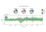
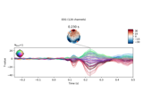
- plot_joint(times='peaks', title='', picks=None, exclude='bads', show=True, ts_args=None, topomap_args=None)[source]
Plot evoked data as butterfly plot and add topomaps for time points.
Note
Axes to plot in can be passed by the user through
ts_argsortopomap_args. In that case bothts_argsandtopomap_argsaxes have to be used. Be aware that when the axes are provided, their position may be slightly modified.- Parameters
- times
float|arrayoffloat| “auto” | “peaks” The time point(s) to plot. If
"auto", 5 evenly spaced topographies between the first and last time instant will be shown. If"peaks", finds time points automatically by checking for 3 local maxima in Global Field Power. Defaults to"peaks".- title
str|None The title. If
None, suppress printing channel type title. If an empty string, a default title is created. Defaults to ‘’. If custom axes are passed make sure to settitle=None, otherwise some of your axes may be removed during placement of the title axis.- picks
str|list|slice|None Channels to include. Slices and lists of integers will be interpreted as channel indices. In lists, channel type strings (e.g.,
['meg', 'eeg']) will pick channels of those types, channel name strings (e.g.,['MEG0111', 'MEG2623']will pick the given channels. Can also be the string values “all” to pick all channels, or “data” to pick data channels. None (default) will pick all channels. Note that channels ininfo['bads']will be included if their names or indices are explicitly provided.- exclude
None|listofstr| ‘bads’ Channels names to exclude from being shown. If
'bads', the bad channels are excluded. Defaults toNone.- showbool
Show figure if
True. Defaults toTrue.- ts_args
None|dict A dict of
kwargsthat are forwarded tomne.Evoked.plot()to style the butterfly plot. If they are not in this dict, the following defaults are passed:spatial_colors=True,zorder='std'.showandexcludeare illegal. IfNone, no customizable arguments will be passed. Defaults toNone.- topomap_args
None|dict A dict of
kwargsthat are forwarded tomne.Evoked.plot_topomap()to style the topomaps. If it is not in this dict,outlines='skirt'will be passed.show,times,colorbarare illegal. IfNone, no customizable arguments will be passed. Defaults toNone.
- times
- Returns
- figinstance of
matplotlib.figure.Figure|list The figure object containing the plot. If
evokedhas multiple channel types, a list of figures, one for each channel type, is returned.
- figinstance of
Notes
New in version 0.12.0.
Examples using
plot_joint:
- plot_projs_topomap(ch_type=None, cmap=None, sensors=True, colorbar=False, res=64, size=1, show=True, outlines='head', contours=6, image_interp='bilinear', axes=None, vlim=(None, None), sphere=None, extrapolate='auto', border='mean')[source]
Plot SSP vector.
- Parameters
- ch_type‘mag’ | ‘grad’ | ‘planar1’ | ‘planar2’ | ‘eeg’ |
None|list The channel type to plot. For ‘grad’, the gradiometers are collec- ted in pairs and the RMS for each pair is plotted. If None (default), it will return all channel types present. If a list of ch_types is provided, it will return multiple figures.
- cmapmatplotlib colormap | (colormap, bool) | ‘interactive’ |
None Colormap to use. If tuple, the first value indicates the colormap to use and the second value is a boolean defining interactivity. In interactive mode (only works if
colorbar=True) the colors are adjustable by clicking and dragging the colorbar with left and right mouse button. Left mouse button moves the scale up and down and right mouse button adjusts the range. Hitting space bar resets the range. Up and down arrows can be used to change the colormap. If None (default), ‘Reds’ is used for all positive data, otherwise defaults to ‘RdBu_r’. If ‘interactive’, translates to (None, True).- sensorsbool |
str Add markers for sensor locations to the plot. Accepts matplotlib plot format string (e.g., ‘r+’ for red plusses). If True, a circle will be used (via .add_artist). Defaults to True.
- colorbarbool
Plot a colorbar.
- res
int The resolution of the topomap image (n pixels along each side).
- sizescalar
Side length of the topomaps in inches (only applies when plotting multiple topomaps at a time).
- showbool
Show figure if True.
- outlines‘head’ | ‘skirt’ |
dict|None The outlines to be drawn. If ‘head’, the default head scheme will be drawn. If ‘skirt’ the head scheme will be drawn, but sensors are allowed to be plotted outside of the head circle. If dict, each key refers to a tuple of x and y positions, the values in ‘mask_pos’ will serve as image mask. Alternatively, a matplotlib patch object can be passed for advanced masking options, either directly or as a function that returns patches (required for multi-axis plots). If None, nothing will be drawn. Defaults to ‘head’.
- contours
int|arrayoffloat The number of contour lines to draw. If 0, no contours will be drawn. When an integer, matplotlib ticker locator is used to find suitable values for the contour thresholds (may sometimes be inaccurate, use array for accuracy). If an array, the values represent the levels for the contours. Defaults to 6.
- image_interp
str The image interpolation to be used. All matplotlib options are accepted.
- axesinstance of
Axes|list|None The axes to plot to. If list, the list must be a list of Axes of the same length as the number of projectors. If instance of Axes, there must be only one projector. Defaults to None.
- vlim
tupleof length 2 | ‘joint’ Colormap limits to use. If
tuple, specifies the lower and upper bounds of the colormap (in that order); providingNonefor either of these will set the corresponding boundary at the min/max of the data (separately for each projector). The keyword value'joint'will compute the colormap limits jointly across all provided projectors of the same channel type, using the min/max of the projector data. If vlim is'joint',infomust not beNone. Defaults to(None, None).- sphere
float| array_like |str|None The sphere parameters to use for the cartoon head. Can be array-like of shape (4,) to give the X/Y/Z origin and radius in meters, or a single float to give the radius (origin assumed 0, 0, 0). Can also be a spherical ConductorModel, which will use the origin and radius. Can be “auto” to use a digitization-based fit. Can also be None (default) to use ‘auto’ when enough extra digitization points are available, and 0.095 otherwise. Currently the head radius does not affect plotting.
New in version 0.20.
- extrapolate
str Options:
'box'Extrapolate to four points placed to form a square encompassing all data points, where each side of the square is three times the range of the data in the respective dimension.
'local'(default)Extrapolate only to nearby points (approximately to points closer than median inter-electrode distance). This will also set the mask to be polygonal based on the convex hull of the sensors.
'head'Extrapolate out to the edges of the clipping circle. This will be on the head circle when the sensors are contained within the head circle, but it can extend beyond the head when sensors are plotted outside the head circle.
Changed in version 0.21:
The default was changed to
'local''local'was changed to use a convex hull mask'head'was changed to extrapolate out to the clipping circle.
New in version 0.20.
- border
float| ‘mean’ Value to extrapolate to on the topomap borders. If
'mean'(default), then each extrapolated point has the average value of its neighbours.New in version 0.20.
- ch_type‘mag’ | ‘grad’ | ‘planar1’ | ‘planar2’ | ‘eeg’ |
- Returns
- figinstance of
Figure Figure distributing one image per channel across sensor topography.
- figinstance of
Examples using
plot_projs_topomap:
- plot_sensors(kind='topomap', ch_type=None, title=None, show_names=False, ch_groups=None, to_sphere=True, axes=None, block=False, show=True, sphere=None, verbose=None)[source]
Plot sensor positions.
- Parameters
- kind
str Whether to plot the sensors as 3d, topomap or as an interactive sensor selection dialog. Available options ‘topomap’, ‘3d’, ‘select’. If ‘select’, a set of channels can be selected interactively by using lasso selector or clicking while holding control key. The selected channels are returned along with the figure instance. Defaults to ‘topomap’.
- ch_type
None|str The channel type to plot. Available options ‘mag’, ‘grad’, ‘eeg’, ‘seeg’, ‘dbs’, ‘ecog’, ‘all’. If
'all', all the available mag, grad, eeg, seeg, dbs, and ecog channels are plotted. If None (default), then channels are chosen in the order given above.- title
str|None Title for the figure. If None (default), equals to
'Sensor positions (%s)' % ch_type.- show_namesbool |
arrayofstr Whether to display all channel names. If an array, only the channel names in the array are shown. Defaults to False.
- ch_groups‘position’ |
arrayof shape (n_ch_groups, n_picks) |None Channel groups for coloring the sensors. If None (default), default coloring scheme is used. If ‘position’, the sensors are divided into 8 regions. See
orderkwarg ofmne.viz.plot_raw(). If array, the channels are divided by picks given in the array.New in version 0.13.0.
- to_spherebool
Whether to project the 3d locations to a sphere. When False, the sensor array appears similar as to looking downwards straight above the subject’s head. Has no effect when kind=’3d’. Defaults to True.
New in version 0.14.0.
- axesinstance of
Axes| instance ofAxes3D|None Axes to draw the sensors to. If
kind='3d', axes must be an instance of Axes3D. If None (default), a new axes will be created.New in version 0.13.0.
- blockbool
Whether to halt program execution until the figure is closed. Defaults to False.
New in version 0.13.0.
- showbool
Show figure if True. Defaults to True.
- sphere
float| array_like |str|None The sphere parameters to use for the cartoon head. Can be array-like of shape (4,) to give the X/Y/Z origin and radius in meters, or a single float to give the radius (origin assumed 0, 0, 0). Can also be a spherical ConductorModel, which will use the origin and radius. Can be “auto” to use a digitization-based fit. Can also be None (default) to use ‘auto’ when enough extra digitization points are available, and 0.095 otherwise. Currently the head radius does not affect plotting.
New in version 0.20.
- verbosebool,
str,int, orNone If not None, override default verbose level (see
mne.verbose()and Logging documentation for more). If used, it should be passed as a keyword-argument only. Defaults to self.verbose.
- kind
- Returns
See also
Notes
This function plots the sensor locations from the info structure using matplotlib. For drawing the sensors using mayavi see
mne.viz.plot_alignment().New in version 0.12.0.
Examples using
plot_sensors:
- plot_topo(layout=None, layout_scale=0.945, color=None, border='none', ylim=None, scalings=None, title=None, proj=False, vline=[0.0], fig_background=None, merge_grads=False, legend=True, axes=None, background_color='w', noise_cov=None, exclude='bads', show=True)[source]
Plot 2D topography of evoked responses.
Clicking on the plot of an individual sensor opens a new figure showing the evoked response for the selected sensor.
- Parameters
- layoutinstance of
Layout|None Layout instance specifying sensor positions (does not need to be specified for Neuromag data). If possible, the correct layout is inferred from the data.
- layout_scale
float Scaling factor for adjusting the relative size of the layout on the canvas.
- color
listof color | color |None Everything matplotlib accepts to specify colors. If not list-like, the color specified will be repeated. If None, colors are automatically drawn.
- border
str Matplotlib borders style to be used for each sensor plot.
- ylim
dict|None Y limits for plots (after scaling has been applied). The value determines the upper and lower subplot limits. e.g. ylim = dict(eeg=[-20, 20]). Valid keys are eeg, mag, grad, misc. If None, the ylim parameter for each channel type is determined by the minimum and maximum peak.
- scalings
dict|None The scalings of the channel types to be applied for plotting. If None,` defaults to
dict(eeg=1e6, grad=1e13, mag=1e15).- title
str Title of the figure.
- projbool | ‘interactive’
If true SSP projections are applied before display. If ‘interactive’, a check box for reversible selection of SSP projection vectors will be shown.
- vline
listoffloat|None The values at which to show a vertical line.
- fig_background
None|ndarray A background image for the figure. This must work with a call to plt.imshow. Defaults to None.
- merge_gradsbool
Whether to use RMS value of gradiometer pairs. Only works for Neuromag data. Defaults to False.
- legendbool |
int|str|tuple If True, create a legend based on evoked.comment. If False, disable the legend. Otherwise, the legend is created and the parameter value is passed as the location parameter to the matplotlib legend call. It can be an integer (e.g. 0 corresponds to upper right corner of the plot), a string (e.g. ‘upper right’), or a tuple (x, y coordinates of the lower left corner of the legend in the axes coordinate system). See matplotlib documentation for more details.
- axesinstance of matplotlib
Axes|None Axes to plot into. If None, axes will be created.
- background_colorcolor
Background color. Typically ‘k’ (black) or ‘w’ (white; default).
New in version 0.15.0.
- noise_covinstance of
Covariance|str|None Noise covariance used to whiten the data while plotting. Whitened data channel names are shown in italic. Can be a string to load a covariance from disk.
New in version 0.16.0.
- exclude
listofstr| ‘bads’ Channels names to exclude from the plot. If ‘bads’, the bad channels are excluded. By default, exclude is set to ‘bads’.
- showbool
Show figure if True.
- layoutinstance of
- Returns
- figinstance of
matplotlib.figure.Figure Images of evoked responses at sensor locations.
- figinstance of
Notes
New in version 0.10.0.
Examples using
plot_topo:
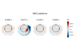
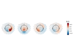
- plot_topomap(times='auto', ch_type=None, vmin=None, vmax=None, cmap=None, sensors=True, colorbar=True, scalings=None, units=None, res=64, size=1, cbar_fmt='%3.1f', time_unit='s', time_format=None, proj=False, show=True, show_names=False, title=None, mask=None, mask_params=None, outlines='head', contours=6, image_interp='bilinear', average=None, axes=None, extrapolate='auto', sphere=None, border='mean', nrows=1, ncols='auto')[source]
Plot topographic maps of specific time points of evoked data.
- Parameters
- times
float|arrayoffloat| “auto” | “peaks” | “interactive” The time point(s) to plot. If “auto”, the number of
axesdetermines the amount of time point(s). Ifaxesis also None, at most 10 topographies will be shown with a regular time spacing between the first and last time instant. If “peaks”, finds time points automatically by checking for local maxima in global field power. If “interactive”, the time can be set interactively at run-time by using a slider.- ch_type
str The channel type being plotted. Determines the
'auto'extrapolation mode.New in version 0.21.
- vmin, vmax
float|callable()|None Lower and upper bounds of the colormap, in the same units as the data. If
vminandvmaxare bothNone, they are set at ± the maximum absolute value of the data (yielding a colormap with midpoint at 0). If only one ofvmin,vmaxisNone, will usemin(data)ormax(data), respectively. If callable, should accept aNumPy arrayof data and return a float.- cmapmatplotlib colormap | (colormap, bool) | ‘interactive’ |
None Colormap to use. If tuple, the first value indicates the colormap to use and the second value is a boolean defining interactivity. In interactive mode the colors are adjustable by clicking and dragging the colorbar with left and right mouse button. Left mouse button moves the scale up and down and right mouse button adjusts the range (zoom). The mouse scroll can also be used to adjust the range. Hitting space bar resets the range. Up and down arrows can be used to change the colormap. If None (default), ‘Reds’ is used for all positive data, otherwise defaults to ‘RdBu_r’. If ‘interactive’, translates to (None, True).
Warning
Interactive mode works smoothly only for a small amount of topomaps. Interactive mode is disabled by default for more than 2 topomaps.
- sensorsbool |
str Add markers for sensor locations to the plot. Accepts matplotlib plot format string (e.g., ‘r+’ for red plusses). If True (default), circles will be used.
- colorbarbool
Plot a colorbar in the rightmost column of the figure.
- scalings
dict|float|None The scalings of the channel types to be applied for plotting. If None, defaults to
dict(eeg=1e6, grad=1e13, mag=1e15).- units
dict|str|None The unit of the channel type used for colorbar label. If scale is None the unit is automatically determined.
- res
int The resolution of the topomap image (n pixels along each side).
- size
float Side length per topomap in inches.
- cbar_fmt
str String format for colorbar values.
- time_unit
str The units for the time axis, can be “ms” or “s” (default).
New in version 0.16.
- time_format
str|None String format for topomap values. Defaults (None) to “%01d ms” if
time_unit='ms', “%0.3f s” iftime_unit='s', and “%g” otherwise. Can be an empty string to omit the time label.- projbool | ‘interactive’ | ‘reconstruct’
If true SSP projections are applied before display. If ‘interactive’, a check box for reversible selection of SSP projection vectors will be shown. If ‘reconstruct’, projection vectors will be applied and then M/EEG data will be reconstructed via field mapping to reduce the signal bias caused by projection.
Changed in version 0.21: Support for ‘reconstruct’ was added.
- showbool
Show figure if True.
- show_namesbool |
callable() If True, show channel names on top of the map. If a callable is passed, channel names will be formatted using the callable; e.g., to delete the prefix ‘MEG ‘ from all channel names, pass the function
lambda x: x.replace('MEG ', ''). Ifmaskis not None, only significant sensors will be shown.- title
str|None Title. If None (default), no title is displayed.
- mask
ndarrayof bool, shape (n_channels, n_times) |None The channels to be marked as significant at a given time point. Indices set to
Truewill be considered. Defaults toNone.- mask_params
dict|None Additional plotting parameters for plotting significant sensors. Default (None) equals:
dict(marker='o', markerfacecolor='w', markeredgecolor='k',
        linewidth=0, markersize=4)
- outlines‘head’ | ‘skirt’ |
dict|None The outlines to be drawn. If ‘head’, the default head scheme will be drawn. If ‘skirt’ the head scheme will be drawn, but sensors are allowed to be plotted outside of the head circle. If dict, each key refers to a tuple of x and y positions, the values in ‘mask_pos’ will serve as image mask. Alternatively, a matplotlib patch object can be passed for advanced masking options, either directly or as a function that returns patches (required for multi-axis plots). If None, nothing will be drawn. Defaults to ‘head’.
- contours
int|arrayoffloat The number of contour lines to draw. If 0, no contours will be drawn. When an integer, matplotlib ticker locator is used to find suitable values for the contour thresholds (may sometimes be inaccurate, use array for accuracy). If an array, the values represent the levels for the contours. The values are in µV for EEG, fT for magnetometers and fT/m for gradiometers. If colorbar=True, the ticks in colorbar correspond to the contour levels. Defaults to 6.
- image_interp
str The image interpolation to be used. All matplotlib options are accepted.
- average
float|None The time window around a given time to be used for averaging (seconds). For example, 0.01 would translate into window that starts 5 ms before and ends 5 ms after a given time point. Defaults to None, which means no averaging.
- axesinstance of
Axes|list|None The axes to plot to. If list, the list must be a list of Axes of the same length as
times(unlesstimesis None). If instance of Axes,timesmust be a float or a list of one float. Defaults to None.- extrapolate
str Options:
'box'Extrapolate to four points placed to form a square encompassing all data points, where each side of the square is three times the range of the data in the respective dimension.
'local'(default)Extrapolate only to nearby points (approximately to points closer than median inter-electrode distance). This will also set the mask to be polygonal based on the convex hull of the sensors.
'head'Extrapolate out to the edges of the clipping circle. This will be on the head circle when the sensors are contained within the head circle, but it can extend beyond the head when sensors are plotted outside the head circle.
Changed in version 0.21:
The default was changed to
'local''local'was changed to use a convex hull mask'head'was changed to extrapolate out to the clipping circle.
New in version 0.18.
- sphere
float| array_like |str|None The sphere parameters to use for the cartoon head. Can be array-like of shape (4,) to give the X/Y/Z origin and radius in meters, or a single float to give the radius (origin assumed 0, 0, 0). Can also be a spherical ConductorModel, which will use the origin and radius. Can be “auto” to use a digitization-based fit. Can also be None (default) to use ‘auto’ when enough extra digitization points are available, and 0.095 otherwise. Currently the head radius does not affect plotting.
New in version 0.20.
- border
float| ‘mean’ Value to extrapolate to on the topomap borders. If
'mean'(default), then each extrapolated point has the average value of its neighbours.New in version 0.20.
- nrows
int| ‘auto’ The number of rows of topographies to plot. Defaults to 1. If ‘auto’, obtains the number of rows depending on the amount of times to plot and the number of cols. Not valid when times == ‘interactive’.
New in version 0.20.
- ncols
int| ‘auto’ The number of columns of topographies to plot. If ‘auto’ (default), obtains the number of columns depending on the amount of times to plot and the number of rows. Not valid when times == ‘interactive’.
New in version 0.20.
- times
- Returns
- figinstance of
matplotlib.figure.Figure The figure.
- figinstance of
Notes
When existing
axesare provided andcolorbar=True, note that the colorbar scale will only accurately reflect topomaps that are generated in the same call as the colorbar. Note also that the colorbar will not be resized automatically whenaxesare provided; use matplotlib’saxes.set_position()method or gridspec interface to adjust the colorbar size yourself.Examples using
plot_topomap:
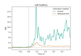
- plot_white(noise_cov, show=True, rank=None, time_unit='s', sphere=None, axes=None, verbose=None)[source]
Plot whitened evoked response.
Plots the whitened evoked response and the whitened GFP as described in 3. This function is especially useful for investigating noise covariance properties to determine if data are properly whitened (e.g., achieving expected values in line with model assumptions, see Notes below).
- Parameters
- noise_cov
list| instance ofCovariance|str The noise covariance. Can be a string to load a covariance from disk.
- showbool
Show figure if True.
- rank
None| ‘info’ | ‘full’ |dict This controls the rank computation that can be read from the measurement info or estimated from the data. When a noise covariance is used for whitening, this should reflect the rank of that covariance, otherwise amplification of noise components can occur in whitening (e.g., often during source localization).
NoneThe rank will be estimated from the data after proper scaling of different channel types.
'info'The rank is inferred from
info. If data have been processed with Maxwell filtering, the Maxwell filtering header is used. Otherwise, the channel counts themselves are used. In both cases, the number of projectors is subtracted from the (effective) number of channels in the data. For example, if Maxwell filtering reduces the rank to 68, with two projectors the returned value will be 66.'full'The rank is assumed to be full, i.e. equal to the number of good channels. If a
Covarianceis passed, this can make sense if it has been (possibly improperly) regularized without taking into account the true data rank.dictCalculate the rank only for a subset of channel types, and explicitly specify the rank for the remaining channel types. This can be extremely useful if you already know the rank of (part of) your data, for instance in case you have calculated it earlier.
This parameter must be a dictionary whose keys correspond to channel types in the data (e.g.
'meg','mag','grad','eeg'), and whose values are integers representing the respective ranks. For example,{'mag': 90, 'eeg': 45}will assume a rank of90and45for magnetometer data and EEG data, respectively.The ranks for all channel types present in the data, but not specified in the dictionary will be estimated empirically. That is, if you passed a dataset containing magnetometer, gradiometer, and EEG data together with the dictionary from the previous example, only the gradiometer rank would be determined, while the specified magnetometer and EEG ranks would be taken for granted.
The default is
None.- time_unit
str The units for the time axis, can be “ms” or “s” (default).
New in version 0.16.
- sphere
float| array_like |str|None The sphere parameters to use for the cartoon head. Can be array-like of shape (4,) to give the X/Y/Z origin and radius in meters, or a single float to give the radius (origin assumed 0, 0, 0). Can also be a spherical ConductorModel, which will use the origin and radius. Can be “auto” to use a digitization-based fit. Can also be None (default) to use ‘auto’ when enough extra digitization points are available, and 0.095 otherwise. Currently the head radius does not affect plotting.
New in version 0.20.
- axes
list|None List of axes to plot into.
New in version 0.21.0.
- verbosebool,
str,int, orNone If not None, override default verbose level (see
mne.verbose()and Logging documentation for more). If used, it should be passed as a keyword-argument only.
- noise_cov
- Returns
- figinstance of
matplotlib.figure.Figure The figure object containing the plot.
- figinstance of
See also
Notes
If baseline signals match the assumption of Gaussian white noise, values should be centered at 0, and be within 2 standard deviations (±1.96) for 95% of the time points. For the global field power (GFP), we expect it to fluctuate around a value of 1.
If one single covariance object is passed, the GFP panel (bottom) will depict different sensor types. If multiple covariance objects are passed as a list, the left column will display the whitened evoked responses for each channel based on the whitener from the noise covariance that has the highest log-likelihood. The left column will depict the whitened GFPs based on each estimator separately for each sensor type. Instead of numbers of channels the GFP display shows the estimated rank. Note. The rank estimation will be printed by the logger (if
verbose=True) for each noise covariance estimator that is passed.References
- 1
Engemann D. and Gramfort A. (2015) Automated model selection in covariance estimation and spatial whitening of MEG and EEG signals, vol. 108, 328-342, NeuroImage.
Examples using
plot_white:
- property proj
Whether or not projections are active.
- rename_channels(mapping, allow_duplicates=False, verbose=None)[source]
Rename channels.
- Parameters
- mapping
dict|callable() A dictionary mapping the old channel to a new channel name e.g. {‘EEG061’ : ‘EEG161’}. Can also be a callable function that takes and returns a string.
Changed in version 0.10.0: Support for a callable function.
- allow_duplicatesbool
If True (default False), allow duplicates, which will automatically be renamed with
-Nat the end.New in version 0.22.0.
- verbosebool,
str,int, orNone If not None, override default verbose level (see
mne.verbose()and Logging documentation for more). If used, it should be passed as a keyword-argument only. Defaults to self.verbose.
- mapping
- Returns
Notes
New in version 0.9.0.
- reorder_channels(ch_names)[source]
Reorder channels.
- Parameters
- ch_names
list The desired channel order.
- ch_names
- Returns
See also
Notes
Channel names must be unique. Channels that are not in
ch_namesare dropped.New in version 0.16.0.
Examples using
reorder_channels:
- resample(sfreq, npad='auto', window='boxcar', n_jobs=1, pad='edge', verbose=None)[source]
Resample data.
If appropriate, an anti-aliasing filter is applied before resampling. See Resampling and decimating data for more information.
Note
Data must be loaded.
- Parameters
- sfreq
float New sample rate to use.
- npad
int|str Amount to pad the start and end of the data. Can also be “auto” to use a padding that will result in a power-of-two size (can be much faster).
- window
str|tuple Frequency-domain window to use in resampling. See
scipy.signal.resample().- n_jobs
int|str Number of jobs to run in parallel. Can be ‘cuda’ if
cupyis installed properly.- pad
str The type of padding to use. Supports all
numpy.pad()modeoptions. Can also be “reflect_limited”, which pads with a reflected version of each vector mirrored on the first and last values of the vector, followed by zeros. Only used formethod='fir'. The default is'edge', which pads with the edge values of each vector.New in version 0.15.
- verbosebool,
str,int, orNone If not None, override default verbose level (see
mne.verbose()and Logging documentation for more). If used, it should be passed as a keyword-argument only. Defaults to self.verbose.
- sfreq
- Returns
See also
Notes
For some data, it may be more accurate to use npad=0 to reduce artifacts. This is dataset dependent – check your data!
Examples using
resample:
- save(fname)[source]
Save dataset to file.
- Parameters
- fname
str The name of the file, which should end with
-ave.fif(.gz)or_ave.fif(.gz).
- fname
Notes
To write multiple conditions into a single file, use
mne.write_evokeds.Changed in version 0.23: Information on baseline correction will be stored with the data, and will be restored when reading again via
mne.read_evokeds.
- savgol_filter(h_freq, verbose=None)[source]
Filter the data using Savitzky-Golay polynomial method.
- Parameters
- h_freq
float Approximate high cut-off frequency in Hz. Note that this is not an exact cutoff, since Savitzky-Golay filtering 4 is done using polynomial fits instead of FIR/IIR filtering. This parameter is thus used to determine the length of the window over which a 5th-order polynomial smoothing is used.
- verbosebool,
str,int, orNone If not None, override default verbose level (see
mne.verbose()and Logging documentation for more). If used, it should be passed as a keyword-argument only. Defaults to self.verbose.
- h_freq
- Returns
See also
Notes
For Savitzky-Golay low-pass approximation, see:
New in version 0.9.0.
References
- 1
Alan V. Oppenheim, Ronald W. Schafer, and John R. Buck. Discrete-Time Signal Processing. Prentice Hall, Upper Saddle River, NJ, 2 edition edition, 1999. ISBN 978-0-13-754920-7.
- 2
Ronald E. Crochiere and Lawrence R. Rabiner. Multirate Digital Signal Processing. Pearson, Englewood Cliffs, NJ, 1 edition edition, 1983. ISBN 978-0-13-605162-6.
- 3
Denis A. Engemann and Alexandre Gramfort. Automated model selection in covariance estimation and spatial whitening of MEG and EEG signals. NeuroImage, 108:328–342, 2015. doi:10.1016/j.neuroimage.2014.12.040.
- 4
Abraham Savitzky and Marcel J. E. Golay. Smoothing and differentiation of data by simplified least squares procedures. Analytical Chemistry, 36(8):1627–1639, 1964. doi:10.1021/ac60214a047.
Examples
>>> import mne
>>> from os import path as op
>>> evoked_fname = op.join(mne.datasets.sample.data_path(), 'MEG', 'sample', 'sample_audvis-ave.fif')
>>> evoked = mne.read_evokeds(evoked_fname, baseline=(None, 0))[0]
>>> evoked.savgol_filter(10.)  # low-pass at around 10 Hz
>>> evoked.plot()
- set_channel_types(mapping, verbose=None)[source]
Define the sensor type of channels.
- Parameters
- mapping
dict A dictionary mapping a channel to a sensor type (str), e.g.,
{'EEG061': 'eog'}.- verbosebool,
str,int, orNone If not None, override default verbose level (see
mne.verbose()and Logging documentation for more). If used, it should be passed as a keyword-argument only. Defaults to self.verbose.
- mapping
- Returns
Notes
The following sensor types are accepted:
ecg, eeg, emg, eog, exci, ias, misc, resp, seeg, dbs, stim, syst, ecog, hbo, hbr, fnirs_cw_amplitude, fnirs_fd_ac_amplitude, fnirs_fd_phase, fnirs_od
New in version 0.9.0.
- set_eeg_reference(ref_channels='average', projection=False, ch_type='auto', forward=None, verbose=None)[source]
Specify which reference to use for EEG data.
Use this function to explicitly specify the desired reference for EEG. This can be either an existing electrode or a new virtual channel. This function will re-reference the data according to the desired reference.
- Parameters
- ref_channels
listofstr|str Can be:
The name(s) of the channel(s) used to construct the reference.
'average'to apply an average reference (default)'REST'to use the Reference Electrode Standardization Technique infinity reference 5.An empty list, in which case MNE will not attempt any re-referencing of the data
- projectionbool
If
ref_channels='average'this argument specifies if the average reference should be computed as a projection (True) or not (False; default). Ifprojection=True, the average reference is added as a projection and is not applied to the data (it can be applied afterwards with theapply_projmethod). Ifprojection=False, the average reference is directly applied to the data. Ifref_channelsis not'average',projectionmust be set toFalse(the default in this case).- ch_type‘auto’ | ‘eeg’ | ‘ecog’ | ‘seeg’ | ‘dbs’
The name of the channel type to apply the reference to. If ‘auto’, the first channel type of eeg, ecog, seeg or dbs that is found (in that order) will be selected.
New in version 0.19.
- forwardinstance of
Forward|None Forward solution to use. Only used with
ref_channels='REST'.New in version 0.21.
- verbosebool,
str,int, orNone If not None, override default verbose level (see
mne.verbose()and Logging documentation for more). If used, it should be passed as a keyword-argument only. Defaults to self.verbose.
- ref_channels
- Returns
See also
mne.set_bipolar_referenceConvenience function for creating bipolar references.
Notes
Some common referencing schemes and the corresponding value for the
ref_channelsparameter:- Average reference:
A new virtual reference electrode is created by averaging the current EEG signal by setting
ref_channels='average'. Bad EEG channels are automatically excluded if they are properly set ininfo['bads'].
- A single electrode:
Set
ref_channelsto a list containing the name of the channel that will act as the new reference, for exampleref_channels=['Cz'].
- The mean of multiple electrodes:
A new virtual reference electrode is created by computing the average of the current EEG signal recorded from two or more selected channels. Set
ref_channelsto a list of channel names, indicating which channels to use. For example, to apply an average mastoid reference, when using the 10-20 naming scheme, setref_channels=['M1', 'M2'].
- REST
The given EEG electrodes are referenced to a point at infinity using the lead fields in
forward, which helps standardize the signals.
If a reference is requested that is not the average reference, this function removes any pre-existing average reference projections.
During source localization, the EEG signal should have an average reference.
In order to apply a reference, the data must be preloaded. This is not necessary if
ref_channels='average'andprojection=True.For an average or REST reference, bad EEG channels are automatically excluded if they are properly set in
info['bads'].
New in version 0.9.0.
References
- 5
D. Yao. A method to standardize a reference of scalp EEG recordings to a point at infinity. Physiological Measurement, 22(4):693–711, 2001. doi:10.1088/0967-3334/22/4/305.
- set_meas_date(meas_date)[source]
Set the measurement start date.
- Parameters
- meas_date
datetime|float|tuple|None The new measurement date. If datetime object, it must be timezone-aware and in UTC. A tuple of (seconds, microseconds) or float (alias for
(meas_date, 0)) can also be passed and a datetime object will be automatically created. If None, will remove the time reference.
- meas_date
- Returns
See also
Notes
If you want to remove all time references in the file, call
mne.io.anonymize_info(inst.info)after callinginst.set_meas_date(None).New in version 0.20.
- set_montage(montage, match_case=True, match_alias=False, on_missing='raise', verbose=None)[source]
Set EEG sensor configuration and head digitization.
- Parameters
- montage
None|str|DigMontage A montage containing channel positions. If str or DigMontage is specified, the channel info will be updated with the channel positions. Default is None. For valid
strvalues see documentation ofmne.channels.make_standard_montage(). See also the documentation ofmne.channels.DigMontagefor more information.- match_casebool
If True (default), channel name matching will be case sensitive.
New in version 0.20.
- match_aliasbool |
dict Whether to use a lookup table to match unrecognized channel location names to their known aliases. If True, uses the mapping in
mne.io.constants.CHANNEL_LOC_ALIASES. If adictis passed, it will be used instead, and should map from non-standard channel names to names in the specifiedmontage. Default isFalse.New in version 0.23.
- on_missing
str Can be
'raise'(default) to raise an error,'warn'to emit a warning, or'ignore'to ignore when channels have missing coordinates.New in version 0.20.1.
- verbosebool,
str,int, orNone If not None, override default verbose level (see
mne.verbose()and Logging documentation for more). If used, it should be passed as a keyword-argument only. Defaults to self.verbose.
- montage
- Returns
Notes
Operates in place.
Examples using
set_montage:
- shift_time(tshift, relative=True)[source]
Shift time scale in epoched or evoked data.
- Parameters
- tshift
float The (absolute or relative) time shift in seconds. If
relativeis True, positive tshift increases the time value associated with each sample, while negative tshift decreases it.- relativebool
If True, increase or decrease time values by
tshiftseconds. Otherwise, shift the time values such that the time of the first sample equalstshift.
- tshift
- Returns
- epochsinstance of
Epochs The modified Epochs instance.
- epochsinstance of
Notes
This method allows you to shift the time values associated with each data sample by an arbitrary amount. It does not resample the signal or change the data values in any way.
Examples using
shift_time:
- time_as_index(times, use_rounding=False)[source]
Convert time to indices.
- Parameters
- Returns
- index
ndarray Indices corresponding to the times supplied.
- index
Examples using
time_as_index:
- property tmax
Last time point.
New in version 0.21.
- property tmin
First time point.
New in version 0.21.
- to_data_frame(picks=None, index=None, scalings=None, copy=True, long_format=False, time_format='ms')[source]
Export data in tabular structure as a pandas DataFrame.
Channels are converted to columns in the DataFrame. By default, an additional column “time” is added, unless
index='time'(in which case time values form the DataFrame’s index).- Parameters
- picks
str|list|slice|None Channels to include. Slices and lists of integers will be interpreted as channel indices. In lists, channel type strings (e.g.,
['meg', 'eeg']) will pick channels of those types, channel name strings (e.g.,['MEG0111', 'MEG2623']will pick the given channels. Can also be the string values “all” to pick all channels, or “data” to pick data channels. None (default) will pick all channels. Note that channels ininfo['bads']will be included if their names or indices are explicitly provided.- index‘time’ |
None Kind of index to use for the DataFrame. If
None, a sequential integer index (pandas.RangeIndex) will be used. If'time', apandas.Float64Index,pandas.Int64Index, orpandas.TimedeltaIndexwill be used (depending on the value oftime_format). Defaults toNone.- scalings
dict|None Scaling factor applied to the channels picked. If
None, defaults todict(eeg=1e6, mag=1e15, grad=1e13)— i.e., converts EEG to µV, magnetometers to fT, and gradiometers to fT/cm.- copybool
If
True, data will be copied. Otherwise data may be modified in place. Defaults toTrue.- long_formatbool
If True, the DataFrame is returned in long format where each row is one observation of the signal at a unique combination of time point and channel. For convenience, a
ch_typecolumn is added to facilitate subsetting the resulting DataFrame. Defaults toFalse.- time_format
str|None Desired time format. If
None, no conversion is applied, and time values remain as float values in seconds. If'ms', time values will be rounded to the nearest millisecond and converted to integers. If'timedelta', time values will be converted topandas.Timedeltavalues. Default is'ms'in version 0.22, and will change toNonein version 0.23.New in version 0.20.
- picks
- Returns
- dfinstance of
pandas.DataFrame A dataframe suitable for usage with other statistical/plotting/analysis packages.
- dfinstance of
Examples using
to_data_frame:
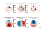
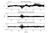
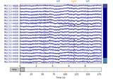
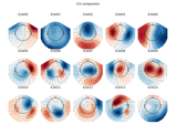
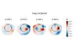
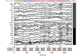
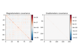
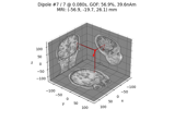
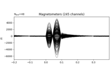
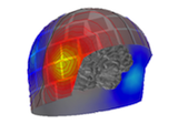
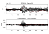
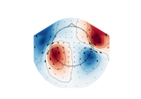
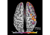
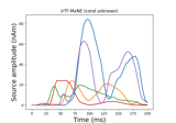
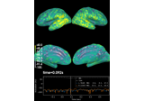
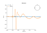
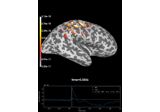
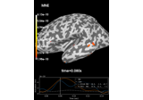
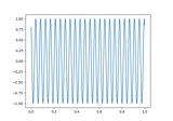
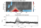
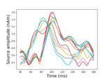
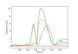
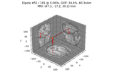

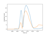
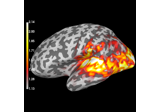
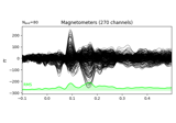
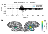
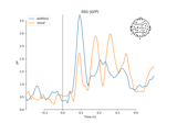

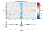
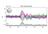
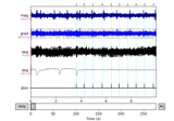
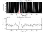
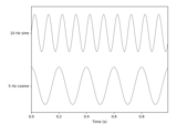
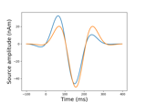
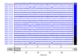
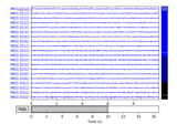
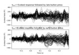
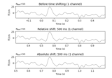
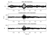
![Regression on continuous data (rER[P/F])](../_images/sphx_glr_linear_regression_raw_thumb.png)