Compute induced power in the source space with dSPM

Returns STC files ie source estimates of induced power for different bands in the source space. The inverse method is linear based on dSPM inverse operator.

# Authors: Alexandre Gramfort <alexandre.gramfort@inria.fr>
#
# License: BSD-3-Clause

import matplotlib.pyplot as plt

import mne
from mne import io
from mne.datasets import sample
from mne.minimum_norm import read_inverse_operator, source_band_induced_power

print(__doc__)

Set parameters

data_path = sample.data_path()
raw_fname = data_path + '/MEG/sample/sample_audvis_raw.fif'
fname_inv = data_path + '/MEG/sample/sample_audvis-meg-oct-6-meg-inv.fif'
tmin, tmax, event_id = -0.2, 0.5, 1

# Setup for reading the raw data
raw = io.read_raw_fif(raw_fname)
events = mne.find_events(raw, stim_channel='STI 014')
inverse_operator = read_inverse_operator(fname_inv)

include = []
raw.info['bads'] += ['MEG 2443', 'EEG 053']  # bads + 2 more

# picks MEG gradiometers
picks = mne.pick_types(raw.info, meg=True, eeg=False, eog=True,
                       stim=False, include=include, exclude='bads')

# Load condition 1
event_id = 1
events = events[:10]  # take 10 events to keep the computation time low
# Use linear detrend to reduce any edge artifacts
epochs = mne.Epochs(raw, events, event_id, tmin, tmax, picks=picks,
                    baseline=(None, 0), reject=dict(grad=4000e-13, eog=150e-6),
                    preload=True, detrend=1)

# Compute a source estimate per frequency band
bands = dict(alpha=[9, 11], beta=[18, 22])

stcs = source_band_induced_power(epochs, inverse_operator, bands, n_cycles=2,
                                 use_fft=False, n_jobs=1)

for b, stc in stcs.items():
    stc.save('induced_power_%s' % b)

Out:

Opening raw data file /home/circleci/mne_data/MNE-sample-data/MEG/sample/sample_audvis_raw.fif...
    Read a total of 3 projection items:
        PCA-v1 (1 x 102)  idle
        PCA-v2 (1 x 102)  idle
        PCA-v3 (1 x 102)  idle
    Range : 25800 ... 192599 =     42.956 ...   320.670 secs
Ready.
320 events found
Event IDs: [ 1  2  3  4  5 32]
Reading inverse operator decomposition from /home/circleci/mne_data/MNE-sample-data/MEG/sample/sample_audvis-meg-oct-6-meg-inv.fif...
    Reading inverse operator info...
    [done]
    Reading inverse operator decomposition...
    [done]
    305 x 305 full covariance (kind = 1) found.
    Read a total of 4 projection items:
        PCA-v1 (1 x 102) active
        PCA-v2 (1 x 102) active
        PCA-v3 (1 x 102) active
        Average EEG reference (1 x 60) active
    Noise covariance matrix read.
    22494 x 22494 diagonal covariance (kind = 2) found.
    Source covariance matrix read.
    22494 x 22494 diagonal covariance (kind = 6) found.
    Orientation priors read.
    22494 x 22494 diagonal covariance (kind = 5) found.
    Depth priors read.
    Did not find the desired covariance matrix (kind = 3)
    Reading a source space...
    Computing patch statistics...
    Patch information added...
    Distance information added...
    [done]
    Reading a source space...
    Computing patch statistics...
    Patch information added...
    Distance information added...
    [done]
    2 source spaces read
    Read a total of 4 projection items:
        PCA-v1 (1 x 102) active
        PCA-v2 (1 x 102) active
        PCA-v3 (1 x 102) active
        Average EEG reference (1 x 60) active
    Source spaces transformed to the inverse solution coordinate frame
Not setting metadata
Not setting metadata
2 matching events found
Setting baseline interval to [-0.19979521315838786, 0.0] sec
Applying baseline correction (mode: mean)
Created an SSP operator (subspace dimension = 3)
3 projection items activated
Loading data for 2 events and 421 original time points ...
0 bad epochs dropped
Preparing the inverse operator for use...
    Scaled noise and source covariance from nave = 1 to nave = 1
    Created the regularized inverter
    Created an SSP operator (subspace dimension = 3)
    Created the whitener using a noise covariance matrix with rank 302 (3 small eigenvalues omitted)
    Computing noise-normalization factors (dSPM)...
[done]
Picked 305 channels from the data
Computing inverse...
    Eigenleads need to be weighted ...
Reducing data rank 305 -> 302
Computing source power ...
[done]
[done]
Writing STC to disk...
[done]
Writing STC to disk...
[done]

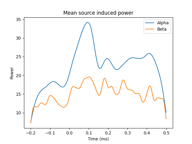
plot mean power

plt.plot(stcs['alpha'].times, stcs['alpha'].data.mean(axis=0), label='Alpha')
plt.plot(stcs['beta'].times, stcs['beta'].data.mean(axis=0), label='Beta')
plt.xlabel('Time (ms)')
plt.ylabel('Power')
plt.legend()
plt.title('Mean source induced power')
plt.show()

Estimated memory usage: 591 MB

previous

Compute source power spectral density (PSD) of VectorView and OPM data

next

Temporal whitening with AR model