Note
Click here to download the full example code
Plotting with mne.viz.Brain
In this example, we’ll show how to use mne.viz.Brain.
# Author: Alex Rockhill <aprockhill@mailbox.org>
#
# License: BSD-3-Clause
Plot a brain
In this example we use the sample data which is data from a subject
being presented auditory and visual stimuli to display the functionality
of mne.viz.Brain for plotting data on a brain.
import os.path as op
import matplotlib.pyplot as plt

import mne
from mne.datasets import sample

print(__doc__)

data_path = sample.data_path()
subjects_dir = op.join(data_path, 'subjects')
sample_dir = op.join(data_path, 'MEG', 'sample')
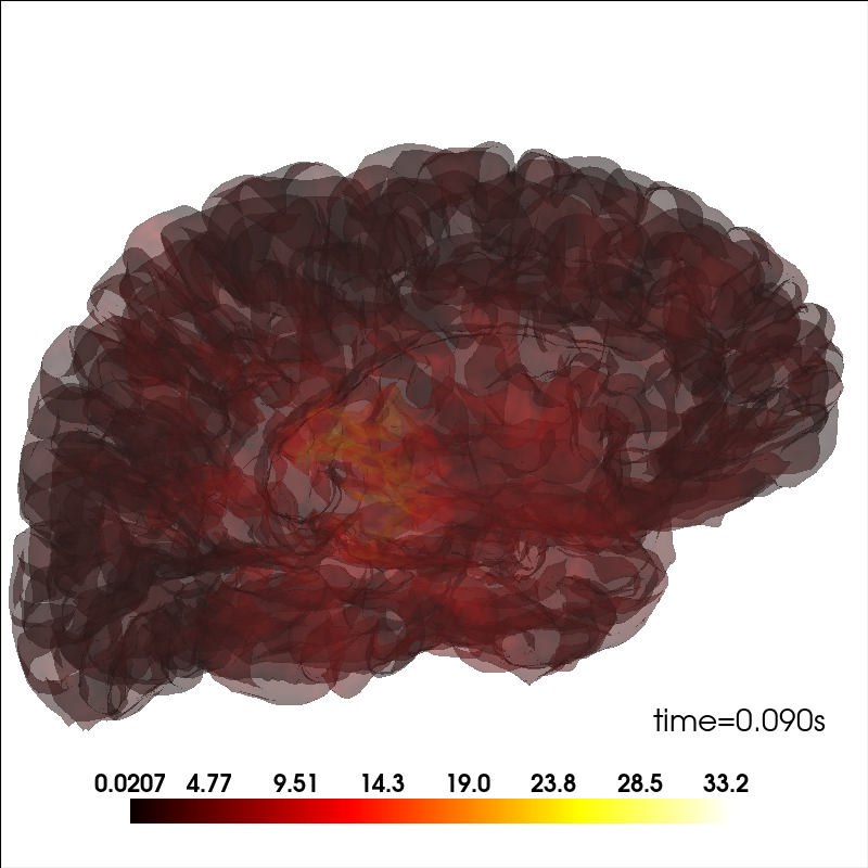
Add source information
Plot source information.
brain_kwargs = dict(alpha=0.1, background='white', cortex='low_contrast')
brain = mne.viz.Brain('sample', subjects_dir=subjects_dir, **brain_kwargs)

stc = mne.read_source_estimate(op.join(sample_dir, 'sample_audvis-meg'))
stc.crop(0.09, 0.1)

kwargs = dict(fmin=stc.data.min(), fmax=stc.data.max(), alpha=0.25,
              smoothing_steps='nearest', time=stc.times)
brain.add_data(stc.lh_data, hemi='lh', vertices=stc.lh_vertno, **kwargs)
brain.add_data(stc.rh_data, hemi='rh', vertices=stc.rh_vertno, **kwargs)
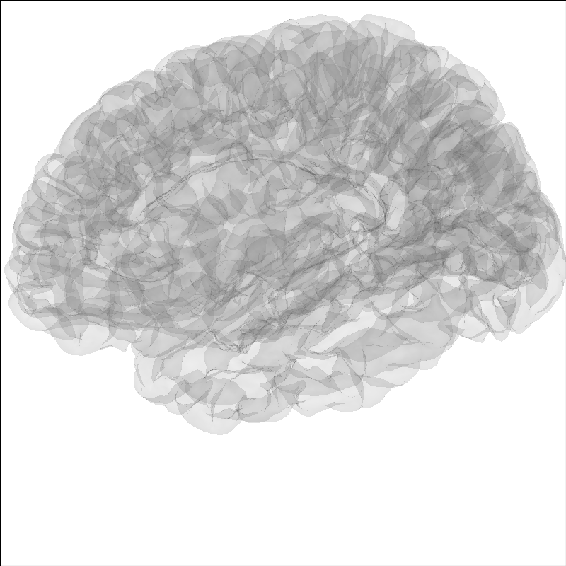
Modify the view of the brain
You can adjust the view of the brain using show_view method.
brain = mne.viz.Brain('sample', subjects_dir=subjects_dir, **brain_kwargs)
brain.show_view(azimuth=190, elevation=70, distance=350, focalpoint=(0, 0, 20))
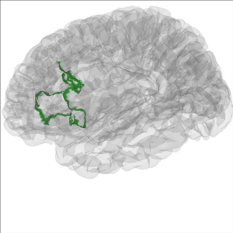
Highlight a region on the brain
It can be useful to highlight a region of the brain for analyses.
To highlight a region on the brain you can use the add_label method.
Labels are stored in the Freesurfer label directory from the recon-all
for that subject. Labels can also be made following the
Freesurfer instructions
Here we will show Brodmann Area 44.
Note
The MNE sample dataset contains only a subselection of the
Freesurfer labels created during the recon-all.
brain = mne.viz.Brain('sample', subjects_dir=subjects_dir, **brain_kwargs)
brain.add_label('BA44', hemi='lh', color='green', borders=True)
brain.show_view(azimuth=190, elevation=70, distance=350, focalpoint=(0, 0, 20))
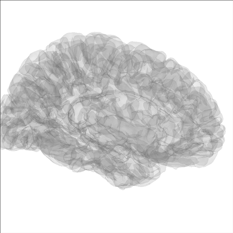
Include the head in the image
Add a head image using the add_head method.
brain = mne.viz.Brain('sample', subjects_dir=subjects_dir, **brain_kwargs)
brain.add_head(alpha=0.5)
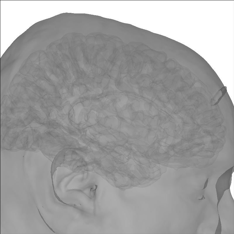
Out:
Using lh.seghead for head surface.
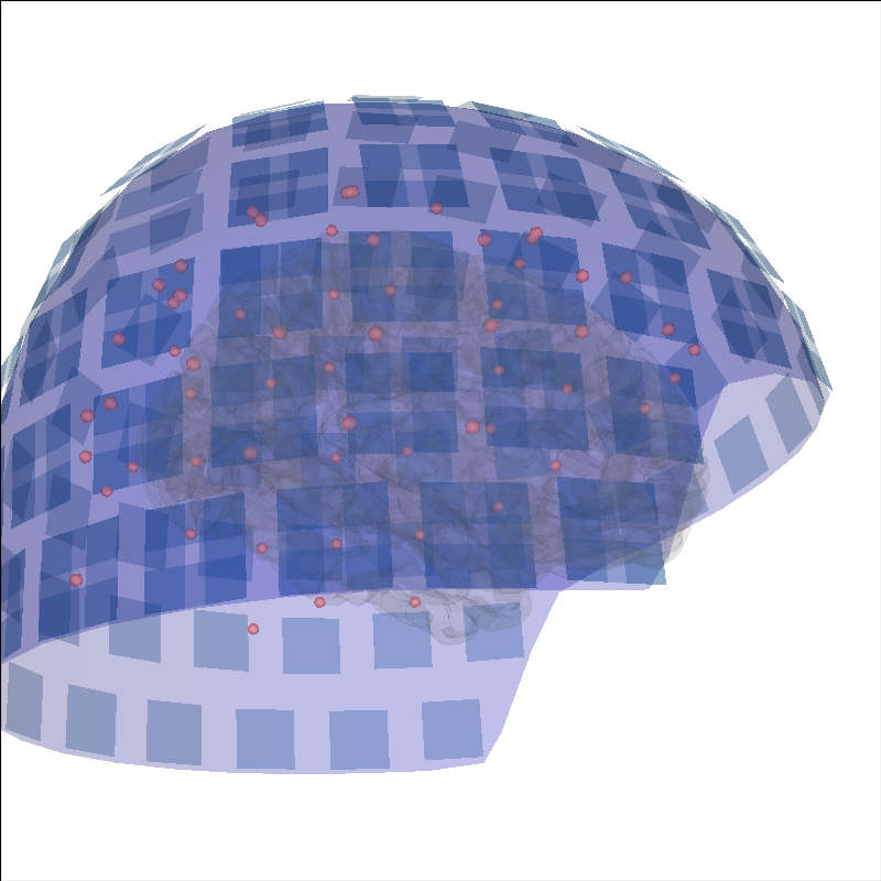
Add sensors positions
To put into context the data that generated the source time course, the sensor positions can be displayed as well.
brain = mne.viz.Brain('sample', subjects_dir=subjects_dir, **brain_kwargs)
evoked = mne.read_evokeds(op.join(sample_dir, 'sample_audvis-ave.fif'))[0]
trans = mne.read_trans(op.join(sample_dir, 'sample_audvis_raw-trans.fif'))
brain.add_sensors(evoked.info, trans)
brain.show_view(distance=500)  # move back to show sensors
Out:
Reading /home/circleci/mne_data/MNE-sample-data/MEG/sample/sample_audvis-ave.fif ...
    Read a total of 4 projection items:
        PCA-v1 (1 x 10²) active
        PCA-v2 (1 x 10²) active
        PCA-v3 (1 x 10²) active
        Average EEG reference (1 x 60) active
    Found the data of interest:
        t =    -199.80 ...     499.49 ms (Left Auditory)
        0 CTF compensation matrices available
        nave = 55 - aspect type = 100
Projections have already been applied. Setting proj attribute to True.
No baseline correction applied
    Read a total of 4 projection items:
        PCA-v1 (1 x 10²) active
        PCA-v2 (1 x 10²) active
        PCA-v3 (1 x 10²) active
        Average EEG reference (1 x 60) active
    Found the data of interest:
        t =    -199.80 ...     499.49 ms (Right Auditory)
        0 CTF compensation matrices available
        nave = 61 - aspect type = 100
Projections have already been applied. Setting proj attribute to True.
No baseline correction applied
    Read a total of 4 projection items:
        PCA-v1 (1 x 10²) active
        PCA-v2 (1 x 10²) active
        PCA-v3 (1 x 10²) active
        Average EEG reference (1 x 60) active
    Found the data of interest:
        t =    -199.80 ...     499.49 ms (Left visual)
        0 CTF compensation matrices available
        nave = 67 - aspect type = 100
Projections have already been applied. Setting proj attribute to True.
No baseline correction applied
    Read a total of 4 projection items:
        PCA-v1 (1 x 10²) active
        PCA-v2 (1 x 10²) active
        PCA-v3 (1 x 10²) active
        Average EEG reference (1 x 60) active
    Found the data of interest:
        t =    -199.80 ...     499.49 ms (Right visual)
        0 CTF compensation matrices available
        nave = 58 - aspect type = 100
Projections have already been applied. Setting proj attribute to True.
No baseline correction applied
Channel types:: grad: 203, mag: 102, eeg: 59
Getting helmet for system 306m
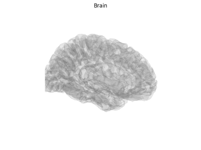
Create a screenshot for exporting the brain image
For publication you may wish to take a static image of the brain,
for this use screenshot.
brain = mne.viz.Brain('sample', subjects_dir=subjects_dir, **brain_kwargs)
img = brain.screenshot()
fig, ax = plt.subplots()
ax.imshow(img)
ax.axis('off')
fig.suptitle('Brain')
Total running time of the script: ( 0 minutes 35.928 seconds)
Estimated memory usage: 27 MB