Note

Click here to download the full example code

Locating Intracranial Electrode Contacts¶

Analysis of intracranial electrophysiology recordings typically involves finding the position of each contact relative to brain structures. In a typical setup, the brain and the electrode locations will be in two places and will have to be aligned; the brain is best visualized by a pre-implantation magnetic resonance (MR) image whereas the electrode contact locations are best visualized in a post-implantation computed tomography (CT) image. The CT image has greater intensity than the background at each of the electrode contacts and for the skull. Using the skull, the CT can be aligned to MR-space. This accomplishes our goal of obtaining contact locations in MR-space (which is where the brain structures are best determined using the FreeSurfer MRI reconstruction). Contact locations in MR-space can also be warped to a template space such as fsaverage for group comparisons.

# Authors: Alex Rockhill <aprockhill@mailbox.org>
#          Eric Larson <larson.eric.d@gmail.com>
#
# License: BSD-3-Clause

import os.path as op

import numpy as np
import matplotlib.pyplot as plt

import nibabel as nib
import nilearn.plotting
from dipy.align import resample

import mne
from mne.datasets import fetch_fsaverage

# paths to mne datasets - sample sEEG and FreeSurfer's fsaverage subject
# which is in MNI space
misc_path = mne.datasets.misc.data_path()
sample_path = mne.datasets.sample.data_path()
subjects_dir = op.join(sample_path, 'subjects')

# use mne-python's fsaverage data
fetch_fsaverage(subjects_dir=subjects_dir, verbose=True)  # downloads if needed

Out:

0 files missing from root.txt in /home/circleci/mne_data/MNE-sample-data/subjects
0 files missing from bem.txt in /home/circleci/mne_data/MNE-sample-data/subjects/fsaverage

Aligning the T1 to ACPC¶

For intracranial electrophysiology recordings, the Brain Imaging Data Structure (BIDS) standard requires that coordinates be aligned to the anterior commissure and posterior commissure (ACPC-aligned). Therefore, it is recommended that you do this alignment before finding the positions of the channels in your recording. Doing this will make the “mri” (aka surface RAS) coordinate frame an ACPC coordinate frame. This can be done using Freesurfer’s freeview:

$ freeview $MISC_PATH/seeg/sample_seeg_T1.mgz

And then interact with the graphical user interface:

First, it is recommended to change the cursor style to long, this can be done through the menu options like so:

Freeview -> Preferences -> General -> Cursor style -> Long

Then, the image needs to be aligned to ACPC to look like the image below. This can be done by pulling up the transform popup from the menu like so:

Tools -> Transform Volume

Note

Be sure to set the text entry box labeled RAS (not TkReg RAS) to 0 0 0 before beginning the transform.

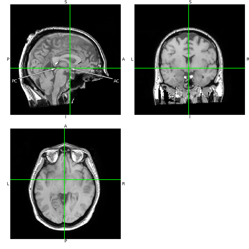
Then translate the image until the crosshairs meet on the AC and run through the PC as shown in the plot. The eyes should be in the ACPC plane and the image should be rotated until they are symmetrical, and the crosshairs should transect the midline of the brain. Be sure to use both the rotate and the translate menus and save the volume after you’re finished using Save Volume As in the transform popup 1.

T1 = nib.load(op.join(misc_path, 'seeg', 'sample_seeg', 'mri', 'T1.mgz'))
viewer = T1.orthoview()
viewer.set_position(0, 9.9, 5.8)
viewer.figs[0].axes[0].annotate(
    'PC', (107, 108), xytext=(10, 75), color='white',
    horizontalalignment='center',
    arrowprops=dict(facecolor='white', lw=0.5, width=2, headwidth=5))
viewer.figs[0].axes[0].annotate(
    'AC', (137, 108), xytext=(246, 75), color='white',
    horizontalalignment='center',
    arrowprops=dict(facecolor='white', lw=0.5, width=2, headwidth=5))

Freesurfer recon-all¶

The first step is the most time consuming; the freesurfer reconstruction. This process segments out the brain from the rest of the MR image and determines which voxels correspond to each brain area based on a template deformation. This process takes approximately 8 hours so plan accordingly.

$ export SUBJECT=sample_seeg
$ export SUBJECTS_DIR=$MY_DATA_DIRECTORY
$ recon-all -subjid $SUBJECT -sd $SUBJECTS_DIR \
  -i $MISC_PATH/seeg/sample_seeg_T1.mgz -all -deface

Note

You may need to include an additional -cw256 flag which can be added to the end of the recon-all command if your MR scan is not 256 x 256 x 256 voxels.

Note

Using the -deface flag will create a defaced, anonymized T1 image located at $MY_DATA_DIRECTORY/$SUBJECT/mri/orig_defaced.mgz, which is helpful for when you publish your data. You can also use mne_bids.write_anat() and pass deface=True.

Aligning the CT to the MR¶

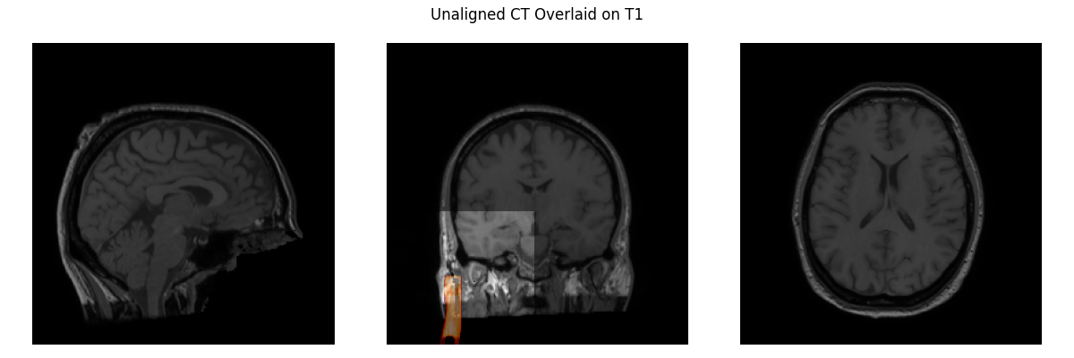
Let’s load our T1 and CT images and visualize them. You can hardly see the CT, it’s so misaligned that it is mostly out of view but there is a part of the skull upsidedown and way off center in the middle plot. Clearly, we need to align the CT to the T1 image.

def plot_overlay(image, compare, title, thresh=None):
    """Define a helper function for comparing plots."""
    image = nib.orientations.apply_orientation(
        np.asarray(image.dataobj), nib.orientations.axcodes2ornt(
            nib.orientations.aff2axcodes(image.affine))).astype(np.float32)
    compare = nib.orientations.apply_orientation(
        np.asarray(compare.dataobj), nib.orientations.axcodes2ornt(
            nib.orientations.aff2axcodes(compare.affine))).astype(np.float32)
    if thresh is not None:
        compare[compare < np.quantile(compare, thresh)] = np.nan
    fig, axes = plt.subplots(1, 3, figsize=(12, 4))
    fig.suptitle(title)
    for i, ax in enumerate(axes):
        ax.imshow(np.take(image, [image.shape[i] // 2], axis=i).squeeze().T,
                  cmap='gray')
        ax.imshow(np.take(compare, [compare.shape[i] // 2],
                          axis=i).squeeze().T, cmap='gist_heat', alpha=0.5)
        ax.invert_yaxis()
        ax.axis('off')
    fig.tight_layout()


CT_orig = nib.load(op.join(misc_path, 'seeg', 'sample_seeg_CT.mgz'))

# resample to T1's definition of world coordinates
CT_resampled = resample(moving=np.asarray(CT_orig.dataobj),
                        static=np.asarray(T1.dataobj),
                        moving_affine=CT_orig.affine,
                        static_affine=T1.affine)
plot_overlay(T1, CT_resampled, 'Unaligned CT Overlaid on T1', thresh=0.95)
del CT_resampled

Now we need to align our CT image to the T1 image.

We want this to be a rigid transformation (just rotation + translation), so we don’t do a full affine registration (that includes shear) here. This takes a while (~10 minutes) to execute so we skip actually running it here:

reg_affine, _ = mne.transforms.compute_volume_registration(
     CT_orig, T1, pipeline='rigids')

And instead we just hard-code the resulting 4x4 matrix:

reg_affine = np.array([
    [0.99270756, -0.03243313, 0.11610254, -133.094156],
    [0.04374389, 0.99439665, -0.09623816, -97.58320673],
    [-0.11233068, 0.10061512, 0.98856381, -84.45551601],
    [0., 0., 0., 1.]])
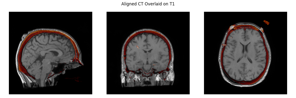
CT_aligned = mne.transforms.apply_volume_registration(CT_orig, T1, reg_affine)
plot_overlay(T1, CT_aligned, 'Aligned CT Overlaid on T1', thresh=0.95)
del CT_orig

Out:

Applying affine registration ...
[done]

We can now see how the CT image looks properly aligned to the T1 image.

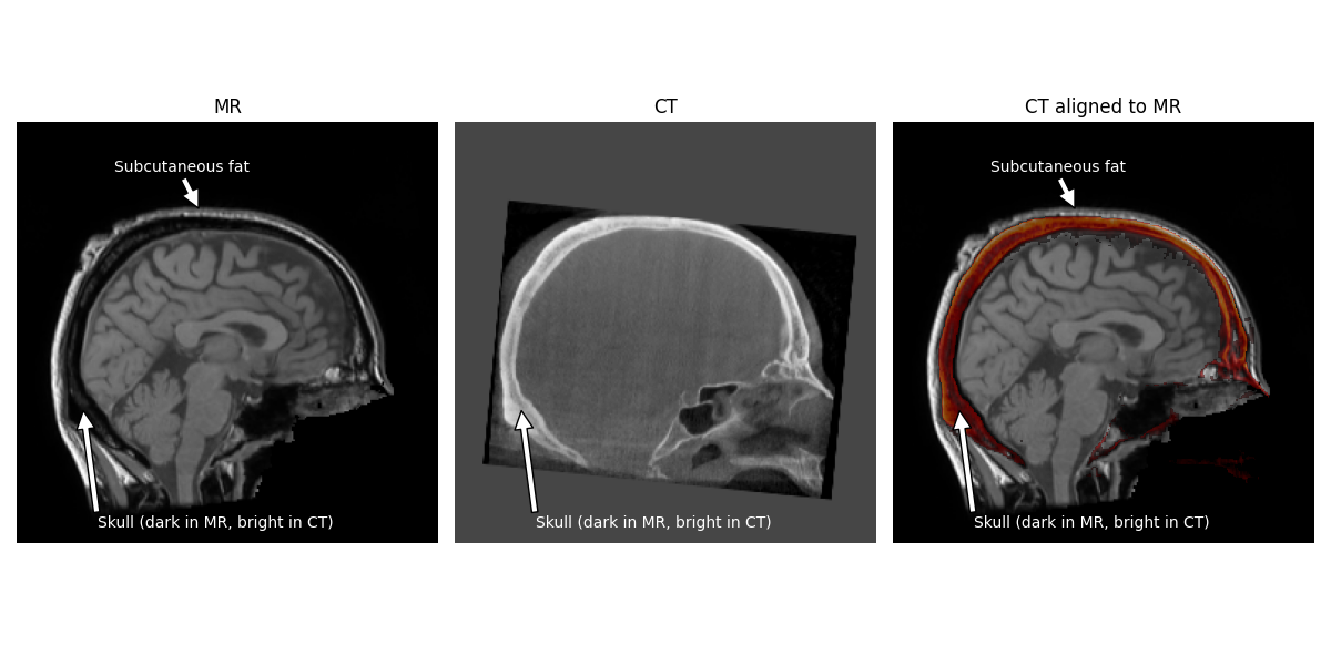
Note

The hyperintense skull is actually aligned to the hypointensity between the brain and the scalp. The brighter area surrounding the skull in the MR is actually subcutaneous fat.

# make low intensity parts of the CT transparent for easier visualization
CT_data = CT_aligned.get_fdata().copy()
CT_data[CT_data < np.quantile(CT_data, 0.95)] = np.nan
T1_data = np.asarray(T1.dataobj)

fig, axes = plt.subplots(1, 3, figsize=(12, 6))
for ax in axes:
    ax.axis('off')
axes[0].imshow(T1_data[T1.shape[0] // 2], cmap='gray')
axes[0].set_title('MR')
axes[1].imshow(np.asarray(CT_aligned.dataobj)[CT_aligned.shape[0] // 2],
               cmap='gray')
axes[1].set_title('CT')
axes[2].imshow(T1_data[T1.shape[0] // 2], cmap='gray')
axes[2].imshow(CT_data[CT_aligned.shape[0] // 2], cmap='gist_heat', alpha=0.5)
for ax in (axes[0], axes[2]):
    ax.annotate('Subcutaneous fat', (110, 52), xytext=(100, 30),
                color='white', horizontalalignment='center',
                arrowprops=dict(facecolor='white'))
for ax in axes:
    ax.annotate('Skull (dark in MR, bright in CT)', (40, 175),
                xytext=(120, 246), horizontalalignment='center',
                color='white', arrowprops=dict(facecolor='white'))
axes[2].set_title('CT aligned to MR')
fig.tight_layout()
del CT_data, T1

Now we need to estimate the “head” coordinate transform.

MNE stores digitization montages in a coordinate frame called “head” defined by fiducial points (origin is halfway between the LPA and RPA see Source alignment and coordinate frames). For sEEG, it is convenient to get an estimate of the location of the fiducial points for the subject using the Talairach transform (see mne.coreg.get_mni_fiducials()) to use to define the coordinate frame so that we don’t have to manually identify their location.

# estimate head->mri transform
subj_trans = mne.coreg.estimate_head_mri_t(
    'sample_seeg', op.join(misc_path, 'seeg'))

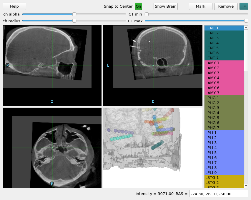
Marking the Location of Each Electrode Contact¶

Now, the CT and the MR are in the same space, so when you are looking at a point in CT space, it is the same point in MR space. So now everything is ready to determine the location of each electrode contact in the individual subject’s anatomical space (T1-space). To do this, we can use the MNE intracranial electrode location graphical user interface.

To operate the GUI:

Click in each image to navigate to each electrode contact

Select the contact name in the right panel

Press the “Mark” button or the “m” key to associate that position with that contact

Repeat until each contact is marked, they will both appear as circles in the plots and be colored in the sidebar when marked

Note

The channel locations are saved to the raw object every time a location is marked or removed so there is no “Save” button.

Note

Using the scroll or +/- arrow keys you can zoom in and out, and the up/down, left/right and page up/page down keys allow you to move one slice in any direction. This information is available in the help menu, accessible by pressing the “h” key.

Note

If “Snap to Center” is on, this will use the radius so be sure to set it properly.

# load electrophysiology data to find channel locations for
# (the channels are already located in the example)
raw = mne.io.read_raw(op.join(misc_path, 'seeg', 'sample_seeg_ieeg.fif'))

gui = mne.gui.locate_ieeg(raw.info, subj_trans, CT_aligned,
                          subject='sample_seeg',
                          subjects_dir=op.join(misc_path, 'seeg'))
# The `raw` object is modified to contain the channel locations
# after closing the GUI and can now be saved
gui.close()  # close when done

Out:

Opening raw data file /home/circleci/mne_data/MNE-misc-data/seeg/sample_seeg_ieeg.fif...
    Range : 1310640 ... 1370605 =   1311.411 ...  1371.411 secs
Ready.

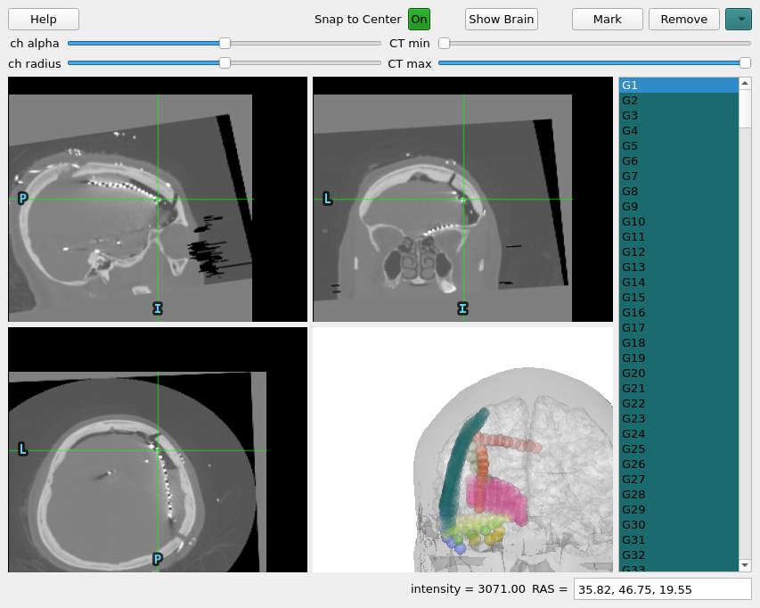
Let’s do a quick sidebar and show what this looks like for ECoG as well.

T1_ecog = nib.load(op.join(misc_path, 'ecog', 'sample_ecog', 'mri', 'T1.mgz'))
CT_orig_ecog = nib.load(op.join(misc_path, 'ecog', 'sample_ecog_CT.mgz'))

# pre-computed affine from `mne.transforms.compute_volume_registration`
reg_affine = np.array([
    [0.99982382, -0.00414586, -0.01830679, 0.15413965],
    [0.00549597, 0.99721885, 0.07432601, -1.54316131],
    [0.01794773, -0.07441352, 0.99706595, -1.84162514],
    [0., 0., 0., 1.]])
# align CT
CT_aligned_ecog = mne.transforms.apply_volume_registration(
    CT_orig_ecog, T1_ecog, reg_affine)

raw_ecog = mne.io.read_raw(op.join(misc_path, 'ecog', 'sample_ecog_ieeg.fif'))
# use estimated `trans` which was used when the locations were found previously
subj_trans_ecog = mne.coreg.estimate_head_mri_t(
    'sample_ecog', op.join(misc_path, 'ecog'))
gui = mne.gui.locate_ieeg(raw_ecog.info, subj_trans_ecog, CT_aligned_ecog,
                          subject='sample_ecog',
                          subjects_dir=op.join(misc_path, 'ecog'))

Out:

Applying affine registration ...
[done]
Opening raw data file /home/circleci/mne_data/MNE-misc-data/ecog/sample_ecog_ieeg.fif...
    Range : 0 ... 112 =      0.000 ...     0.700 secs
Ready.

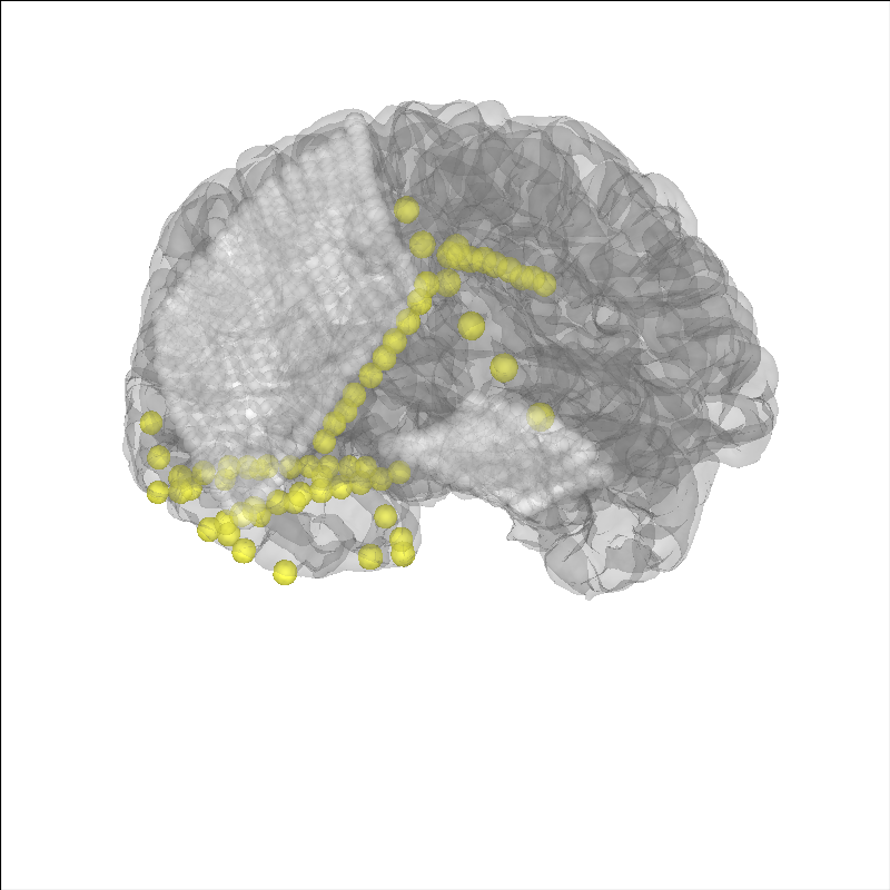
for ECoG, we typically want to account for “brain shift” or shrinking of the brain away from the skull/dura due to changes in pressure during the craniotomy Note: this requires the BEM surfaces to have been computed e.g. using mne watershed_bem or mne flash_bem. First, let’s plot the localized sensor positions without modification.

# plot projected sensors
brain_kwargs = dict(cortex='low_contrast', alpha=0.2, background='white')
brain = mne.viz.Brain('sample_ecog', subjects_dir=op.join(misc_path, 'ecog'),
                      title='Before Projection', **brain_kwargs)
brain.add_sensors(raw_ecog.info, trans=subj_trans_ecog)
view_kwargs = dict(azimuth=60, elevation=100, distance=350,
                   focalpoint=(0, 0, -15))
brain.show_view(**view_kwargs)

Out:

Channel types:: ecog: 320, seeg: 74

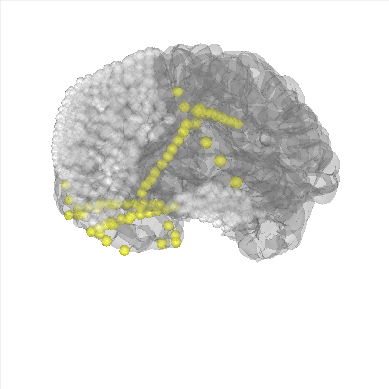
Now, let’s project the sensors to the brain surface and re-plot them.

# project sensors to the brain surface
raw_ecog.info = mne.preprocessing.ieeg.project_sensors_onto_brain(
    raw_ecog.info, subj_trans_ecog, 'sample_ecog',
    subjects_dir=op.join(misc_path, 'ecog'))

# plot projected sensors
brain = mne.viz.Brain('sample_ecog', subjects_dir=op.join(misc_path, 'ecog'),
                      title='After Projection', **brain_kwargs)
brain.add_sensors(raw_ecog.info, trans=subj_trans_ecog)
brain.show_view(**view_kwargs)

Out:

Channel types:: ecog: 320, seeg: 74

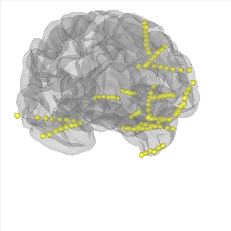
Let’s plot the electrode contact locations on the subject’s brain.

# plot the alignment
brain = mne.viz.Brain('sample_seeg', subjects_dir=op.join(misc_path, 'seeg'),
                      **brain_kwargs)
brain.add_sensors(raw.info, trans=subj_trans)
brain.show_view(**view_kwargs)

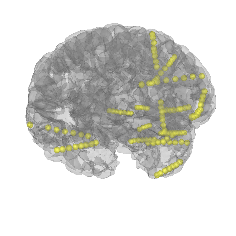
Out:

Channel types:: seeg: 119

Warping to a Common Atlas¶

Electrode contact locations are often compared across subjects in a template space such as fsaverage or cvs_avg35_inMNI152. To transform electrode contact locations to that space, we need to determine a function that maps from the subject’s brain to the template brain. We will use the symmetric diffeomorphic registration (SDR) implemented by Dipy to do this.

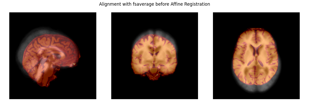
Before we can make a function to account for individual differences in the shape and size of brain areas, we need to fix the alignment of the brains. The plot below shows that they are not yet aligned.

# load the subject's brain and the Freesurfer "fsaverage" template brain
subject_brain = nib.load(
    op.join(misc_path, 'seeg', 'sample_seeg', 'mri', 'brain.mgz'))
template_brain = nib.load(
    op.join(subjects_dir, 'fsaverage', 'mri', 'brain.mgz'))

plot_overlay(template_brain, subject_brain,
             'Alignment with fsaverage before Affine Registration')

Alignment with fsaverage before Affine Registration

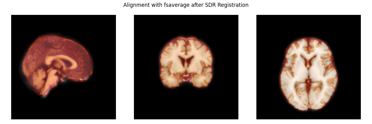
Now, we’ll register the affine of the subject’s brain to the template brain. This aligns the two brains, preparing the subject’s brain to be warped to the template.

Warning

Here we use custom zooms just for speed, in general we recommend using zooms=None (default) for highest accuracy!

zooms = dict(translation=4, rigid=4, affine=6, sdr=6)
reg_affine, sdr_morph = mne.transforms.compute_volume_registration(
    subject_brain, template_brain, zooms=zooms, verbose=True)
subject_brain_sdr = mne.transforms.apply_volume_registration(
    subject_brain, template_brain, reg_affine, sdr_morph)

# apply the transform to the subject brain to plot it
plot_overlay(template_brain, subject_brain_sdr,
             'Alignment with fsaverage after SDR Registration')

del subject_brain, template_brain

Alignment with fsaverage after SDR Registration

Out:

Computing registration...
Reslicing to zooms=(4.0, 4.0, 4.0) for translation ...
Optimizing translation:
    Optimizing level 2 [max iter: 10000]
    Optimizing level 1 [max iter: 1000]
    Optimizing level 0 [max iter: 100]
    Translation:    4.7 mm
    R²:            94.5%
Optimizing rigid:
    Optimizing level 2 [max iter: 10000]
    Optimizing level 1 [max iter: 1000]
    Optimizing level 0 [max iter: 100]
    Translation:    7.0 mm
    Rotation:      15.3°
    R²:            96.1%
Reslicing to zooms=(6.0, 6.0, 6.0) for affine ...
Optimizing affine:
    Optimizing level 2 [max iter: 10000]
    Optimizing level 1 [max iter: 1000]
    Optimizing level 0 [max iter: 100]
    R²:            95.5%
Optimizing sdr:
    R²:            98.2%
Applying affine registration ...
Appling SDR warp ...
[done]

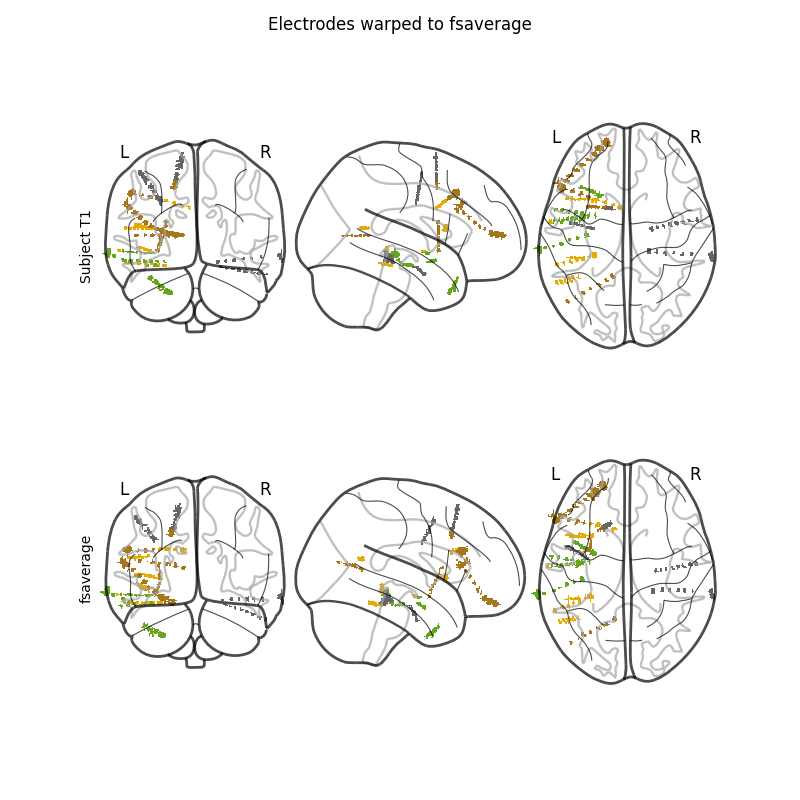
Finally, we’ll apply the registrations to the electrode contact coordinates. The brain image is warped to the template but the goal was to warp the positions of the electrode contacts. To do that, we’ll make an image that is a lookup table of the electrode contacts. In this image, the background will be 0 s all the bright voxels near the location of the first contact will be 1 s, the second 2 s and so on. This image can then be warped by the SDR transform. We can finally recover a position by averaging the positions of all the voxels that had the contact’s lookup number in the warped image.

# first we need our montage but it needs to be converted to "mri" coordinates
# using our ``subj_trans``
montage = raw.get_montage()
montage.apply_trans(subj_trans)

montage_warped, elec_image, warped_elec_image = mne.warp_montage_volume(
    montage, CT_aligned, reg_affine, sdr_morph, thresh=0.25,
    subject_from='sample_seeg', subjects_dir_from=op.join(misc_path, 'seeg'),
    subject_to='fsaverage', subjects_dir_to=subjects_dir)

fig, axes = plt.subplots(2, 1, figsize=(8, 8))
nilearn.plotting.plot_glass_brain(elec_image, axes=axes[0], cmap='Dark2')
fig.text(0.1, 0.65, 'Subject T1', rotation='vertical')
nilearn.plotting.plot_glass_brain(warped_elec_image, axes=axes[1],
                                  cmap='Dark2')
fig.text(0.1, 0.25, 'fsaverage', rotation='vertical')
fig.suptitle('Electrodes warped to fsaverage')

del CT_aligned

Out:

Applying affine registration ...
Appling SDR warp ...
[done]

We can now plot the result. You can compare this to the plot in Working with sEEG data to see the difference between this morph, which is more complex, and the less-complex, linear Talairach transformation. By accounting for the shape of this particular subject’s brain using the SDR to warp the positions of the electrode contacts, the position in the template brain is able to be more accurately estimated.

# first we need to add fiducials so that we can define the "head" coordinate
# frame in terms of them (with the origin at the center between LPA and RPA)
montage_warped.add_estimated_fiducials('fsaverage', subjects_dir)

# compute the head<->mri ``trans`` now using the fiducials
template_trans = mne.channels.compute_native_head_t(montage_warped)

# now we can set the montage and, because there are fiducials in the montage,
# the montage will be properly transformed to "head" coordinates when we do
# (this step uses ``template_trans`` but it is recomputed behind the scenes)
raw.set_montage(montage_warped)

# plot the resulting alignment
brain = mne.viz.Brain('fsaverage', subjects_dir=subjects_dir, **brain_kwargs)
brain.add_sensors(raw.info, trans=template_trans)
brain.show_view(**view_kwargs)

Out:

Channel types:: seeg: 119

This pipeline was developed based on previous work 1.

References¶

1(1,2): Liberty S. Hamilton, David L. Chang, Morgan B. Lee, and Edward F. Chang. Semi-automated anatomical labeling and inter-subject warping of high-density intracranial recording electrodes in electrocorticography. Frontiers in Neuroinformatics, October 2017. URL: http://journal.frontiersin.org/article/10.3389/fninf.2017.00062/full, doi:10.3389/fninf.2017.00062.

Total running time of the script: ( 1 minutes 59.162 seconds)

Estimated memory usage: 989 MB

Gallery generated by Sphinx-Gallery

Decoding (MVPA)

Working with sEEG data