Custom DSS: Defining Your Own Bias.

This example demonstrates how to extend DSS by defining custom bias criteria. This is useful when you have domain-specific knowledge about the target source (e.g., “it has sharp gradients”, “it occurs after a specific trigger”, etc.).

It shows two ways to define custom biases: subclassing LinearDenoiser for full control over the bias computation, and using function-based weighting ideas for simpler auxiliary-data strategies.

Here, we implement a Gradient Trigger Bias that finds sources with sharp transients (high temporal gradient) by weighting time points where the gradient magnitude is high.

Authors: Sina Esmaeili (sina.esmaeili@umontreal.ca)

Hamza Abdelhedi (hamza.abdelhedi@umontreal.ca)

import matplotlib.pyplot as plt
import numpy as np
from scipy import signal

from mne_denoise.dss import DSS, LinearDenoiser

Part 1: Defining a Custom Bias Class

To define a custom linear bias, we subclass mne_denoise.dss.LinearDenoiser. We must implement the compute_bias(data) method, which returns the covariance matrix of the “biased” (filtered/weighted) data.

class GradientTriggerBias(LinearDenoiser):
    """
    Custom IDSS Bias that emphasizes signals with sharp gradients.

    It weights the covariance matrix based on the magnitude of the
    temporal gradient of the data.

    Parameters
    ----------
    threshold : float
        Percentile (0-100) of gradient magnitude to keep.
        Only time points with gradient > percentile are used.
    """

    def __init__(self, threshold_percentile=90):
        self.threshold_percentile = threshold_percentile

    def apply(self, data):
        """
        Apply bias transformation to data.

        Parameters
        ----------
        data : ndarray, shape (n_channels, n_times)
            The input data (usually whitened).

        Returns
        -------
        biased_data : ndarray, shape (n_channels, n_times)
            The biased data (weighted by gradient).
        """
        # 1. Compute temporal gradient (approximate derivative)
        # diff(data, axis=1) gives (n_ch, n_times-1)
        grad = np.diff(data, axis=1, prepend=data[:, :1])

        # 2. Compute gradient magnitude (energy across channels) at each time point
        # sum of squares across channels
        grad_energy = np.sum(grad**2, axis=0)

        # 3. Determine threshold
        thresh = np.percentile(grad_energy, self.threshold_percentile)

        # 4. Create a mask (float for multiplication)
        # We keep time points where gradient energy is high
        mask = (grad_energy > thresh).astype(float)

        print(
            f"  GradientTriggerBias: Weighting "
            f"{np.sum(mask)} / {len(mask)} samples "
            f"({mask.mean() * 100:.1f}%)"
        )

        # 5. Return weighted data
        # Covariance C_bias will later be computed as (biased_data @ biased_data.T) / N
        return data * mask

Part 2: Generating Synthetic Data with Transients

We create a dataset with a transient source made of rare sharp spikes, a background source made of a smooth 10 Hz oscillation, and additive Gaussian white noise.

n_samples = 2000
time = np.arange(n_samples) / 200.0  # 200 Hz

# Source 1: Sharp Transients (The Target)
s1 = np.zeros(n_samples)
# Add random spikes
rng = np.random.default_rng(42)
spike_indices = rng.choice(n_samples, 20, replace=False)
s1[spike_indices] = 5.0  # Impulses
# Convolve with a sharp kernel to make them "transients" but not single-sample
kernel = signal.windows.exponential(20, tau=3.0)
s1 = np.convolve(s1, kernel, mode="same")
s1 /= s1.std()

# Source 2: Smooth Background (Distractor)
# We make it slower (2 Hz) so its gradient is lower than the sharp transients
s2 = np.sin(2 * np.pi * 2 * time)
s2 /= s2.std()

# Source 3: Removed (White noise has too high gradient!)
# We only use Target and Distractor for clear demonstration
# s3 = rng.standard_normal(n_samples)

S = np.array([s1, s2])
n_sources = S.shape[0]

# Mixing
A = rng.standard_normal((5, n_sources))
X = A @ S
# Add sensor noise
X += 0.1 * rng.standard_normal(X.shape)

print(f"Synthesized Data: {X.shape} (5 channels, 2000 samples)")

# Plot Input
fig, axes = plt.subplots(3, 1, figsize=(10, 6), sharex=True)
axes[0].plot(time, s1, "r")
axes[0].set_title("Target Source (Transients)")
axes[1].plot(time, s2, "k")
axes[1].set_title("Distractor Source (Smooth 10Hz)")
axes[2].plot(time, X[0], "gray")
axes[2].set_title("Mixed Sensor Signal (Ch 0)")
plt.tight_layout()
plt.show()

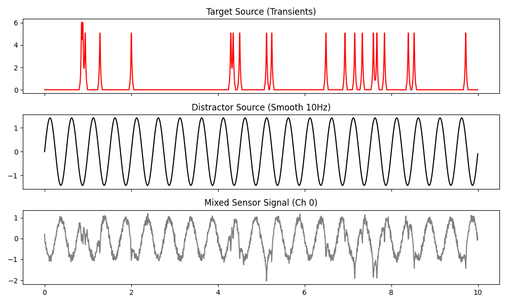
Synthesized Data: (5, 2000) (5 channels, 2000 samples)

Part 3: Applying the Custom Bias

We plug our GradientTriggerBias into DSS.

print("\n--- Running DSS with Custom GradientTriggerBias ---")

# We want to find the component that has the most energy *during high gradients*
custom_bias = GradientTriggerBias(threshold_percentile=95)

dss = DSS(bias=custom_bias, n_components=3)
dss.fit(X)
S_est = dss.transform(X)

# Plot Results
fig, axes = plt.subplots(3, 1, figsize=(10, 6), sharex=True)
axes[0].plot(time, S_est[0], "r")
axes[0].set_title("DSS Component 0 (Biased to Gradients)")
axes[1].plot(time, S_est[1], "k")
axes[1].set_title("DSS Component 1")
axes[2].plot(time, S_est[2], "b")
axes[2].set_title("DSS Component 2")
axes[-1].set_xlabel("Time (s)")
plt.suptitle("Custom Bias Results")
plt.tight_layout()
plt.show()

# Check correlation with target
corr = np.abs(np.corrcoef(S_est[0], s1)[0, 1])
print(f"Correlation between Component 0 and Target Transients: {corr:.3f}")

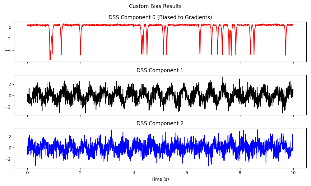
--- Running DSS with Custom GradientTriggerBias ---
  GradientTriggerBias: Weighting 100.0 / 2000 samples (5.0%)
Correlation between Component 0 and Target Transients: 0.997

Part 4: Using function_bias (Functional API)

For simpler cases where you just want to weight the covariance matrix by some weighting vector w(t), you don’t need to subclass. You can use a closure.

Concept: covariance C = sum( w[t] * x[t] * x[t].T )

Let’s say we have an auxiliary channel (e.g., a microphone or trigger channel) and we want to bias towards times where this channel is active.

print("\n--- Using Functional Approach (Simple Wrapper) ---")

# Create a dummy "trigger" channel that aligns with the spikes
# In reality, this would be your aux channel.
aux_trigger = np.abs(s1)  # We cheat and use the envelope of s1 as our 'weight'


# Define a function wrapper class (since we removed function_bias helper)
class FunctionalBias(LinearDenoiser):
    def __init__(self, weights):
        self.weights = weights

    def apply(self, data):
        # Weight the data (sqrt(weights) because Cov = X @ X.T)
        # But for simpler Power weighting, we just multiply
        # Ensure weights align
        return data * self.weights


dss_func = DSS(bias=FunctionalBias(aux_trigger), n_components=3)
dss_func.fit(X)
S_func = dss_func.transform(X)

fig, ax = plt.subplots(figsize=(10, 3))
ax.plot(time, S_func[0], "g")
ax.set_title("Functional Bias Result (Weighted by Envelope)")
plt.tight_layout()
print("\nExample 9 Complete!")
plt.show()

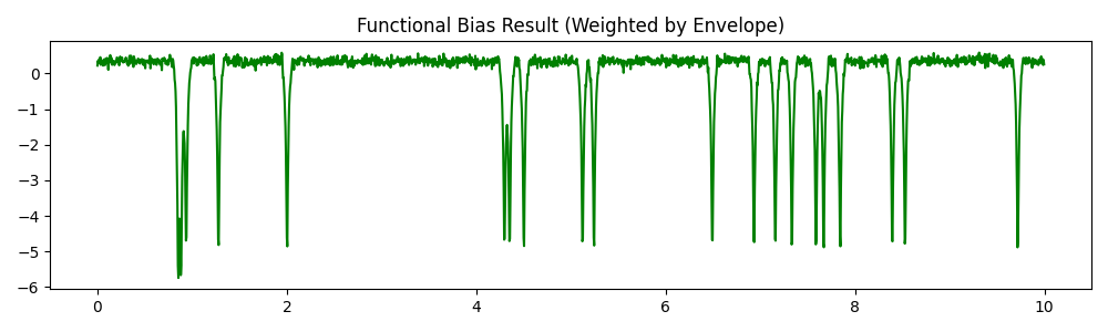
--- Using Functional Approach (Simple Wrapper) ---

Example 9 Complete!