Denoising Evoked Responses.

This example demonstrates how to use DSS to enhance evoked responses (ERPs/ERFs). It covers both standard average-bias denoising of the shared evoked response and a custom contrast bias that isolates the difference between two experimental conditions.

Authors: Sina Esmaeili (sina.esmaeili@umontreal.ca)

Hamza Abdelhedi (hamza.abdelhedi@umontreal.ca)

Imports

import contextlib
import os

import matplotlib.pyplot as plt
import mne
import numpy as np
from mne.datasets import sample

from mne_denoise.dss import DSS, AverageBias, LinearDenoiser
from mne_denoise.viz import (
    plot_component_score_curve,
    plot_component_summary,
    plot_component_time_series,
    plot_evoked_gfp_comparison,
)

Part 0: Synthetic Data Demo

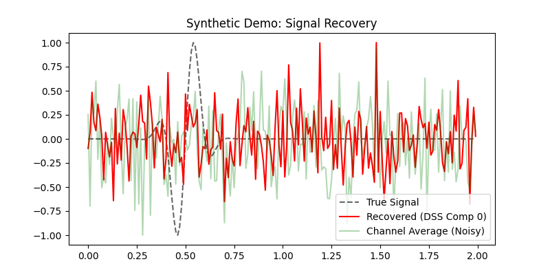
Before using real data, let’s demonstrate the concept on a simple simulation. We create a known “Evoked Response” (damped sinusoid) and bury it in noise.

The goal is to recover the template response from the noisy mixture.

print("\n--- Part 0: Synthetic Data Demo ---")

# 1. Simulate Data
rng = np.random.default_rng(42)
n_epochs = 50
n_channels = 10
n_times = 200
sfreq = 100
times = np.arange(n_times) / sfreq

# Define the "True" Evoked Response (N100-like)
# Peak around 100ms (0.1s)
signal = -np.exp(-((times - 0.5) ** 2) / 0.01) * np.sin(2 * np.pi * 5 * times)
signal /= np.max(np.abs(signal))  # Normalize

# Embed in Epochs
epochs_data = np.zeros((n_epochs, n_channels, n_times))
mixing = rng.standard_normal(n_channels)
mixing /= np.linalg.norm(mixing)
signal_strength = 0.5

for i in range(n_epochs):
    # Noise: non-phase-locked (random every trial)
    noise = rng.standard_normal((n_channels, n_times)) * 2.0
    # Add signal (phase-locked)
    for ch in range(n_channels):
        epochs_data[i, ch, :] = noise[ch] + mixing[ch] * signal * signal_strength

# Create MNE Epochs
info_sim = mne.create_info(n_channels, sfreq, "eeg")
events_sim = np.array([[i * 1000, 0, 1] for i in range(n_epochs)])
epochs_sim = mne.EpochsArray(
    epochs_data, info_sim, events=events_sim, tmin=-0.5, verbose=False
)

# 2. Fit DSS
dss_sim = DSS(n_components=5, bias=AverageBias(axis="epochs"))
dss_sim.fit(epochs_sim)

# 3. Visualize Results
# Plot true signal vs First DSS component
# DSS component sign is arbitrary, so we match it to the template for comparison
sources_sim = dss_sim.transform(epochs_sim)
evoked_source = sources_sim.mean(axis=0)[0]  # First component, averaged trials
if np.corrcoef(evoked_source, signal)[0, 1] < 0:
    evoked_source *= -1

plt.figure(figsize=(8, 4))
plt.plot(times, signal, "k--", label="True Signal", alpha=0.6)
plt.plot(
    times,
    evoked_source / np.max(np.abs(evoked_source)),
    "r-",
    label="Recovered (DSS Comp 0)",
)
plt.plot(
    times,
    epochs_sim.average().data[0] / np.max(np.abs(epochs_sim.average().data[0])),
    "g-",
    alpha=0.3,
    label="Channel Average (Noisy)",
)
plt.title("Synthetic Demo: Signal Recovery")
plt.legend()
plt.show()

print("Synthetic demo complete. Proceeding to Real Data...\n")

--- Part 0: Synthetic Data Demo ---
/home/runner/work/mne-denoise/mne-denoise/mne_denoise/dss/linear.py:496: RuntimeWarning: Epochs are not baseline corrected, covariance matrix may be inaccurate
  baseline_cov = mne.compute_covariance(inst, method=method, **kws)
/home/runner/work/mne-denoise/mne-denoise/mne_denoise/dss/linear.py:498: RuntimeWarning: Epochs are not baseline corrected, covariance matrix may be inaccurate
  biased_cov = mne.compute_covariance(biased_inst, method=method, **kws)
Synthetic demo complete. Proceeding to Real Data...

Load Data

print("Loading MNE Sample data...")
home = os.path.expanduser("~")
mne_data_path = os.path.join(home, "mne_data")
if not os.path.exists(mne_data_path):
    with contextlib.suppress(OSError):
        os.makedirs(mne_data_path)

data_path = sample.data_path()
raw_fname = data_path / "MEG" / "sample" / "sample_audvis_raw.fif"
raw = mne.io.read_raw_fif(raw_fname, preload=True, verbose=False)
raw.crop(0, 60)  # Keep it short for speed

# Filter to clearer evoked band (1-40 Hz)
raw.filter(1, 40, fir_design="firwin")

# Extract events
events = mne.find_events(raw, stim_channel="STI 014")
event_id = {"Auditory/Left": 1, "Auditory/Right": 2}

# Create Epochs
epochs = mne.Epochs(
    raw,
    events,
    event_id,
    tmin=-0.2,
    tmax=0.5,
    baseline=(None, 0),
    reject={"grad": 4000e-13, "mag": 4e-12, "eog": 150e-6},
    preload=True,
    verbose=False,
)

# Pick MEG data for DSS
epochs_meg = epochs.copy().pick_types(meg=True, eeg=False, eog=False, exclude="bads")
epochs_meg_topomap_picks = mne.pick_types(
    epochs_meg.info, meg="grad", eeg=False, eog=False, exclude="bads"
)
print(f"Epochs: {len(epochs_meg)} trials, {len(epochs_meg.ch_names)} channels")

Loading MNE Sample data...
Filtering raw data in 1 contiguous segment
Setting up band-pass filter from 1 - 40 Hz

FIR filter parameters
---------------------
Designing a one-pass, zero-phase, non-causal bandpass filter:
- Windowed time-domain design (firwin) method
- Hamming window with 0.0194 passband ripple and 53 dB stopband attenuation
- Lower passband edge: 1.00
- Lower transition bandwidth: 1.00 Hz (-6 dB cutoff frequency: 0.50 Hz)
- Upper passband edge: 40.00 Hz
- Upper transition bandwidth: 10.00 Hz (-6 dB cutoff frequency: 45.00 Hz)
- Filter length: 1983 samples (3.302 s)

Finding events on: STI 014
86 events found on stim channel STI 014
Event IDs: [ 1  2  3  4  5 32]
NOTE: pick_types() is a legacy function. New code should use inst.pick(...).
Epochs: 34 trials, 305 channels

Part 1: Standard Evoked Denoising

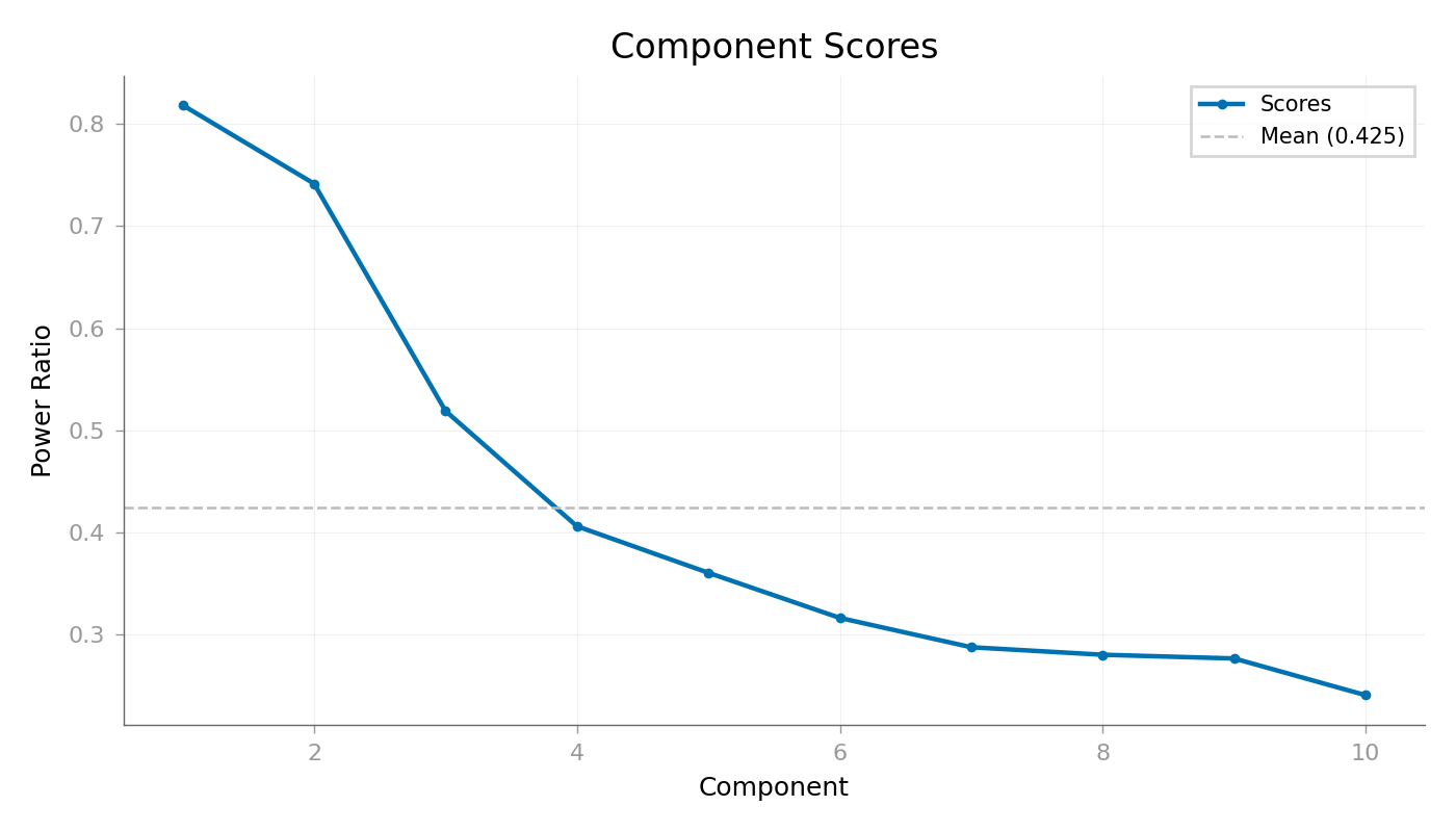
Here the bias is trial reproducibility: components are ranked by how strongly they reflect the evoked response relative to total power.

print("\n--- Part 1: Standard Trial Average Bias ---")

# 1. Fit DSS
# We use AverageBias(axis='epochs'), which replaces every
# trial with the mean of all trials.
dss_std = DSS(
    n_components=10,
    bias=AverageBias(axis="epochs"),
    cov_method="empirical",
    cov_kws={"n_jobs": 1},
)
dss_std.fit(epochs_meg)

# Visualize
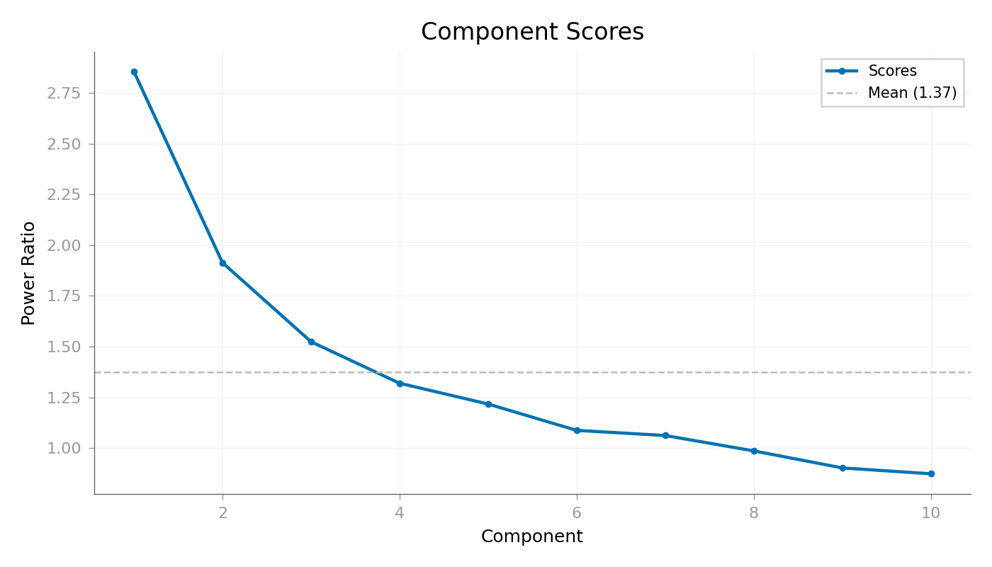
# The score curve shows how "evoked" each component is (0 to 1).
plot_component_score_curve(dss_std, mode="ratio", show=True)

--- Part 1: Standard Trial Average Bias ---

<Figure size 1400x800 with 1 Axes>

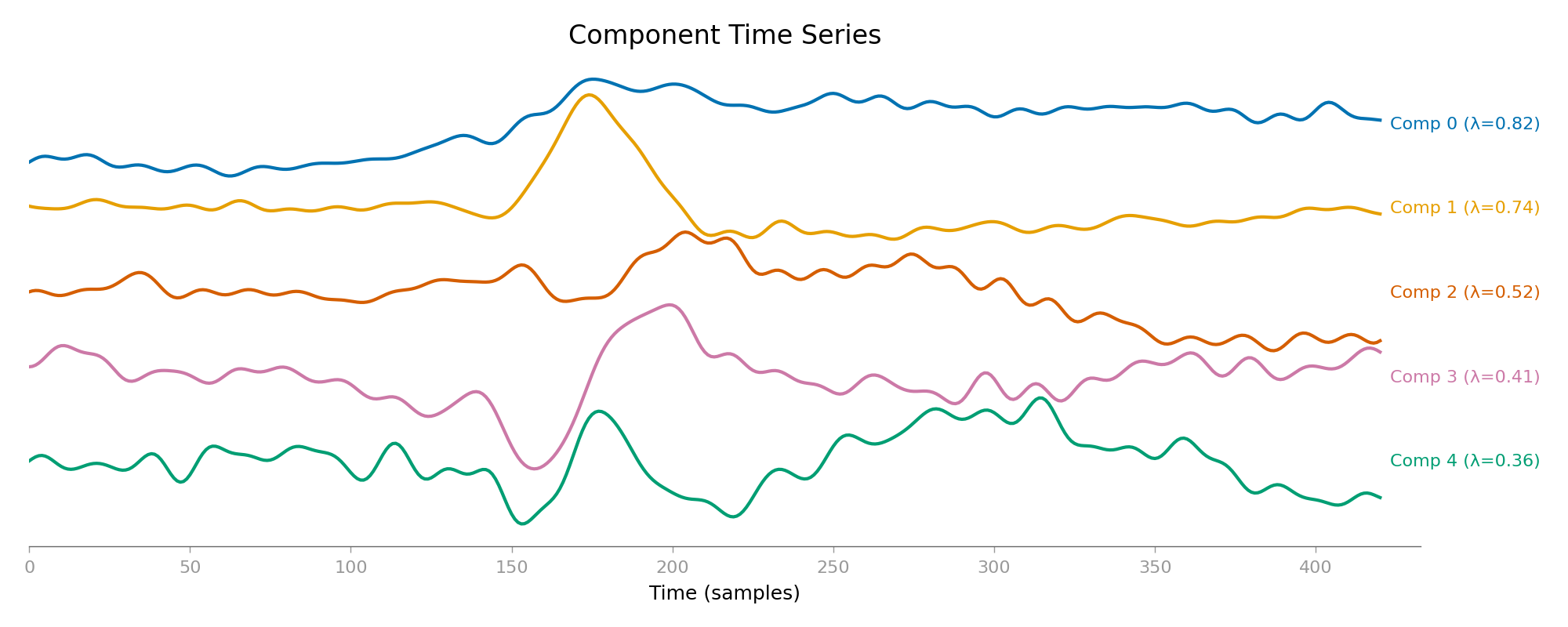
Time Series of top components

plot_component_time_series(dss_std, data=epochs_meg, n_components=5, show=True)

<Figure size 2000x800 with 1 Axes>

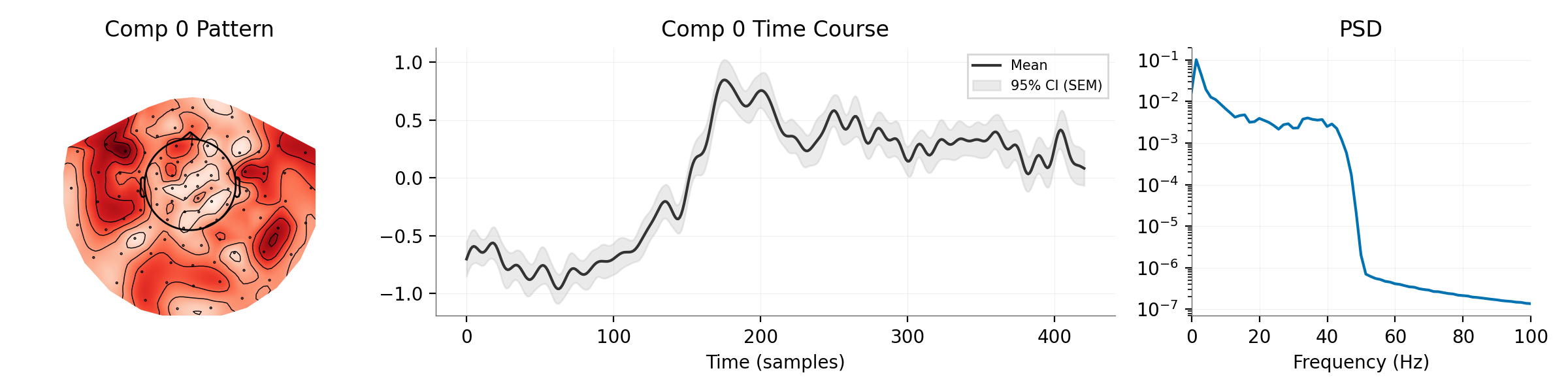
The first component should be the dominant N100 response.

plot_component_summary(
    dss_std,
    data=epochs_meg,
    info=epochs_meg.info,
    picks=epochs_meg_topomap_picks,
    n_components=[0],
    show=True,
)

<Figure size 2400x600 with 3 Axes>

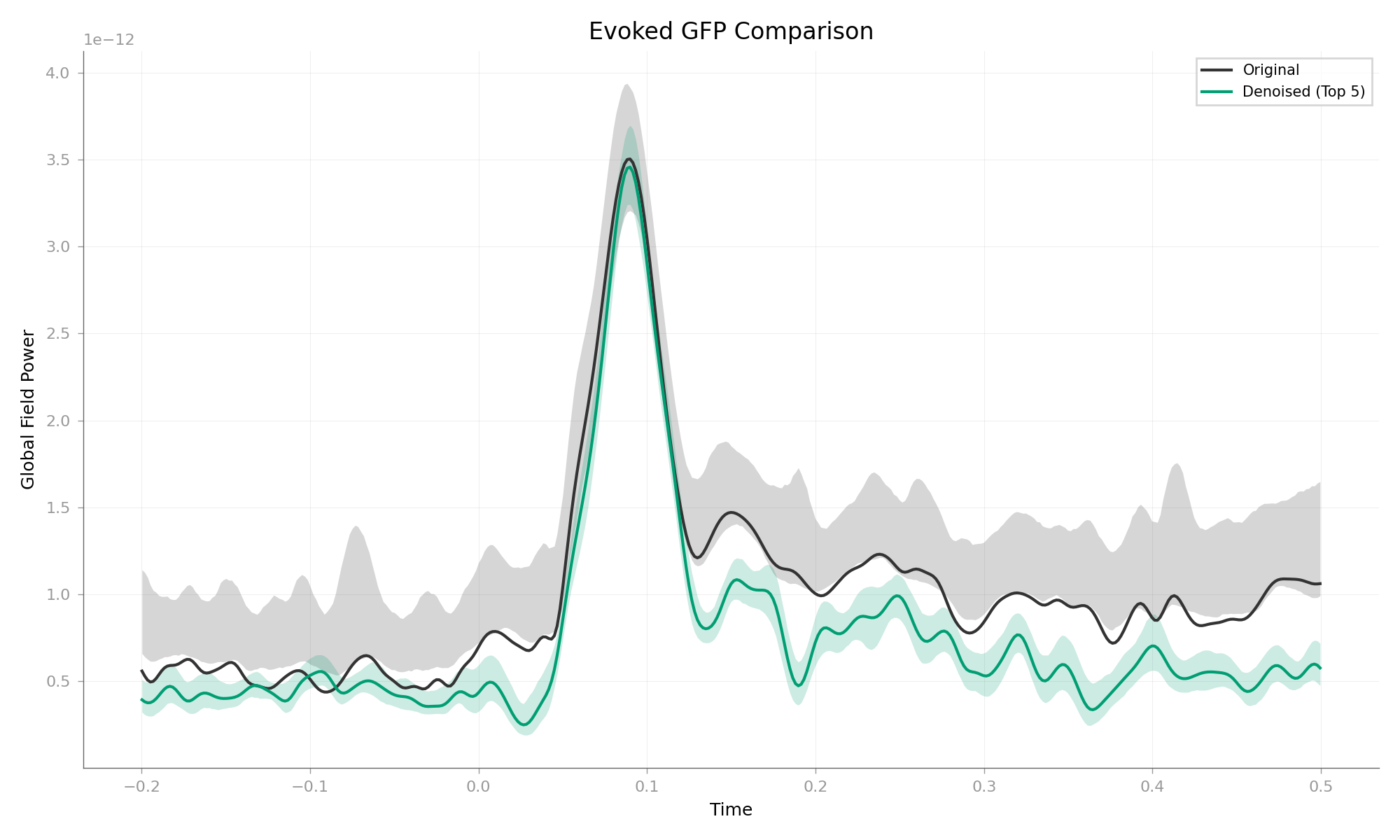
3. Denoising Effect We reconstruct the data using ONLY the top few reproducible components. This removes “non-evoked” background noise (alpha waves, etc. that are not phase-locked).

keep_n = 5
print(f"Reconstructing Evoked with top {keep_n} components...")

# Transform -> Zero out noise -> Inverse
sources = dss_std.transform(epochs_meg)
# Create a mask to keep only top N
mask = np.zeros(dss_std.n_components, dtype=bool)
mask[:keep_n] = True

# Inverse transform (filtering out the rest)
clean_data = dss_std.inverse_transform(sources, component_indices=mask)
epochs_clean = mne.EpochsArray(
    clean_data,
    epochs_meg.info,
    tmin=epochs_meg.tmin,
    events=epochs_meg.events,
    event_id=epochs_meg.event_id,
)

# Compare Global Field Power
plot_evoked_gfp_comparison(
    epochs_meg,
    epochs_clean,
    times=epochs_meg.times,
    labels=("Original", f"Denoised (Top {keep_n})"),
    show=True,
)


# Quantify Improvement (SNR = Peak Evoked Power / Baseline Variance)
def get_snr(ep):
    evoked = ep.average()
    gfp = np.std(evoked.data, axis=0)  # spatial std (GFP)
    # SNR = Peak post-stim / Mean pre-stim
    return np.max(gfp[ep.times > 0]) / np.mean(gfp[ep.times < 0])


snr_in = get_snr(epochs_meg)
snr_out = get_snr(epochs_clean)
print(
    f"SNR Improvement: {snr_in:.2f} -> {snr_out:.2f} "
    f"({snr_out / snr_in:.1f}x improvement)"
)

Reconstructing Evoked with top 5 components...
Not setting metadata
34 matching events found
No baseline correction applied
Created an SSP operator (subspace dimension = 3)
3 projection items activated
SNR Improvement: 6.72 -> 8.03 (1.2x improvement)

Part 2: Custom Contrast Bias (Oddball / Difference)

A contrast bias shifts the target from repeatability alone to the difference between two conditions, which is useful when the scientific question is condition-specific rather than purely evoked.

print("\n--- Part 2: Custom Contrast Bias ---")


# Define Custom Bias Class
class ContrastBias(LinearDenoiser):
    """Enhance the difference between two conditions."""

    def __init__(self, events, id_a, id_b):
        self.events = events
        self.id_a = id_a
        self.id_b = id_b

    def apply(self, data):
        # data shape: (n_channels, n_times, n_epochs)
        # Note: 'data' passed to apply is usually the full epoch data matrix
        # We need to know which epoch belongs to which condition.
        # Ideally, we pass 'events' to init so we can index.

        # Identify indices
        idx_a = [i for i, evt in enumerate(self.events) if evt[2] == self.id_a]
        idx_b = [i for i, evt in enumerate(self.events) if evt[2] == self.id_b]

        if len(idx_a) == 0 or len(idx_b) == 0:
            raise ValueError("Events for Condition A or B not found in data.")

        # Compute means
        # data is (n_ch, n_times, n_epochs)
        mean_a = data[:, :, idx_a].mean(axis=2)
        mean_b = data[:, :, idx_b].mean(axis=2)

        # The 'Biased' signal is the Difference Wave
        diff = mean_a - mean_b

        # We start with a zero array
        biased = np.zeros_like(data)

        # For this bias, we want to maximize power in the difference.
        # So we replace *every* trial with the difference wave.
        # (Or we could replace A trials with +Diff/2 and B trials with -Diff/2,
        #  but projecting onto the simple Difference vector is robust).
        biased = np.broadcast_to(diff[:, :, np.newaxis], data.shape).copy()

        return biased


# 1. Setup Custom Bias
# Left (1) vs Right (2)
custom_bias = ContrastBias(epochs_meg.events, id_a=1, id_b=2)

# 2. Fit DSS
dss_diff = DSS(
    n_components=10, bias=custom_bias, cov_method="empirical", cov_kws={"n_jobs": 1}
)
dss_diff.fit(epochs_meg)

# 3. Visualize
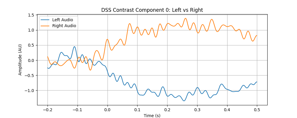
# Component 0 should be the "Difference Component".
plot_component_score_curve(dss_diff, mode="ratio", show=True)

--- Part 2: Custom Contrast Bias ---

<Figure size 1400x800 with 1 Axes>

Let’s plot the time series of Comp 0 for Left vs Right conditions separate. We expect to see a strong separation.

src_diff = dss_diff.transform(epochs_meg)  # (n_epochs, n_comps, n_times)

# Average by condition
src_left = src_diff[epochs_meg.events[:, 2] == 1].mean(axis=0)
src_right = src_diff[epochs_meg.events[:, 2] == 2].mean(axis=0)

times = epochs_meg.times
plt.figure(figsize=(10, 4))
plt.plot(times, src_left[0], label="Left Audio", color="tab:blue")
plt.plot(times, src_right[0], label="Right Audio", color="tab:orange")
plt.title("DSS Contrast Component 0: Left vs Right")
plt.xlabel("Time (s)")
plt.ylabel("Amplitude (AU)")
plt.legend()
plt.grid(True)
plt.show()

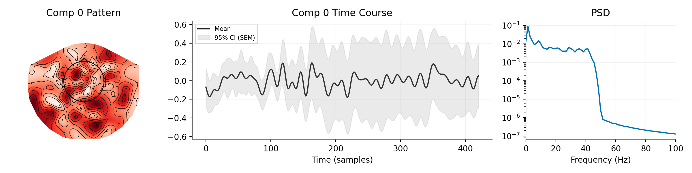
4. Topography of the Difference This topography explains the difference between left and right.

plot_component_summary(
    dss_diff,
    data=epochs_meg,
    info=epochs_meg.info,
    picks=epochs_meg_topomap_picks,
    n_components=[0],
    show=True,
)

<Figure size 2400x600 with 3 Axes>